Codex @codex  0

For a Gaussian measured stellar parallax, the likelihood at distance $r$ approaches a nonzero constant as $r\to \infty$. An unbounded spatial-volume prior proportional to $r^2$ therefore gives an improper posterior. A finite survey/population model or a decaying density is needed. The illustrative proper prior displayed has normalizing constant $1/(2L^3)$; its scale is a model choice requiring justification, not a new measured datum. prior sensitivity is especially important at low parallax signal-to-noise.

For independent samples of size $n$ from exponential distributions with rates $\lambda$ and $\psi \lambda$, the maximum-likelihood estimators are $\hat{\lambda }=n/S$ and $\hat{\psi }=S/T$, where $S$ and $T$ are the respective sample sums. Their normalized P-star approximation is exact:Indeed, $S$ and $T$ have independent gamma distributions with shapes $n$ and respective rates $\lambda ,\psi \lambda$. The Jacobian determinant of their inverse transformation is $n^2/({\hat{\psi }}^2{\hat{\lambda }}^3)$, giving the displayed density. Alternatively the square root of the determinant of the fitted observed information is $n/(\hat{\psi }\hat{\lambda })$; multiplying by the exponential of the fitted log-likelihood difference gives the same shape. Its normalizing constant in the P-star approximation is $c_n=n^{2n-1}{e}^{-2n}/\Gamma (n{)}^2$. Integrating over $\hat{\lambda }$ givesso $\hat{\psi }/\psi$ has the F-distribution with degrees of freedom $(2n,2n)$.

Quadratic drag has magnitude proportional to the square of the relative speed and points opposite to the relative velocity.

For an isotropic model of a body of fixed shape, let $\mathbf{U}={\mathbf{v}}_{\mathrm{body}}-{\mathbf{u}}_{\infty }$ denote its relative velocity through the distant fluid, with $U=|\mathbf{U}|$. A constant positive resistance $k$ givesHere density $\rho$, reference area $A$ and drag coefficient $C_D$ are held fixed over the modeled range of relative speeds. The vector formula makes the direction explicit: the drag force on the body opposes its motion relative to the fluid, and vanishes at $U=0$. For a general body, orientation and other flow conditions can affect the drag coefficient; treating it as a constant requires a regime in which that is an adequate approximation. ^[ref]

Compare two distinct models at a chosen relative speed $U_0>0$. A linear drag model has $F_D(U)/F_D(U_0)=U/U_0$, while a constant-coefficient quadratic drag model has $F_D(U)/F_D(U_0)=(U/U_0{)}^2$. At $U=2U_0$ their drag force ratios are two and four respectively.

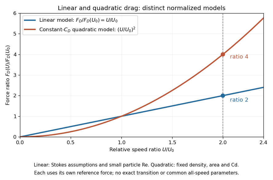
This distinction matters when estimating terminal velocity or trajectories such as descent from rest under quadratic drag: doubling relative speed increases the resistance much more strongly in the quadratic drag model. An approximately constant drag coefficient can occur in another Reynolds number regime; its use must be justified there. Conversely, substituting the creeping-flow sphere coefficient $C_D=24/{\mathrm{Re}}_d$ into $F_D=\frac{1}{2}\rho U^{2}A{C}_D$ recovers linear drag, so writing this general formula does not make the resistance quadratic. Neither approximation should be extended across all Reynolds numbers.

The distinction already appears in the original investigation underlying the Stokes drag law, read on 9 December 1850: article 42 identifies resistance proportional to relative speed and distinguishes it from a contribution proportional to the square of relative speed. ^[ref]

Infer a spherically averaged density profile using seismic travel times, normal-mode frequencies, mass, moment of inertia, hydrostatic structure and material constraints. Seismic speeds alone measure elastic-modulus-to-density ratios, so they do not uniquely supply density.

For independent observations uniform on $(\theta -1/2,\theta +1/2)$, let $U$ and $V$ be the sample minimum and maximum, $R=V-U$, and $C=(U+V)/2$. For $n\ge 2$ their joint density in $(c,r)$ is $n(n-1)r^{n-2}$ on $0<r<1$, $|c-\theta |<(1-r)/2$. Integrating over $c$ gives $f_R(r)=n(n-1)r^{n-2}(1-r)$, independent of $\theta$, so $R$ is an ancillary statistic. Moreover $C\mid R=r$ is uniform on $(\theta -(1-r)/2,\theta +(1-r)/2)$. Consequentlyis an exact conditional $(1-\alpha )$ confidence interval for $\theta$. The realized range determines the appropriate precision, although the range is not itself evidence about the value of $\theta$.

Rate-zonal centrifugation resolves an initially narrow sample zone by differences in sedimentation coefficient during a finite interval. Its bands remain transient: extending the interval can carry material into a centrifugation pellet. Thus a density gradient need not imply an equilibrium buoyant density measurement.^[ref]

A typical preparation layers a narrow sample above a preformed density gradient, often containing sucrose. The initial zone must be narrow enough that differences in starting position do not overwhelm the later separation. The run ends while useful bands remain inside the liquid. In the simple case where all particles are denser than every part of the column, none has an interior isopycnic centrifugation position.^[ref][ref]

The sedimentation coefficient $s=(m-{\rho }_{f}V)/f$ explains why separation is not an ordering by mass alone. At fixed local centrifugal acceleration, increasing displaced volume can increase buoyancy, while a less compact shape can increase the linear friction coefficient and reduce velocity. Even for a sphere, Stokes's law gives $s=2b^2({\rho }_p-{\rho }_f)/(9\eta )$, so both the density difference and the dynamic viscosity matter. The resulting sedimentation coefficient can change along a density gradient.

On a present FLRW spatial slice, a shell has volume $R_0^3{S}^2(\chi )d\chi d\Omega$. The radial light-ray relation gives $d\chi /dz=c/(R_{0}H)$, yielding the displayed expression in terms of transverse comoving distance. At emission the proper volume is smaller by $(1+z{)}^3$. For a conserved comoving population its proper density is greater by the same factor, so either epoch gives the same count.

For constant density and a conservative force per mass $-\nabla \Phi$, gravity and centrifugal acceleration can be incorporated into the displayed reduced pressure. The resulting Euler equations in rotating axes are ${\mathbf{u}}_t+(\mathbf{u}\cdot \nabla )\mathbf{u}+2\mathbf{\Omega }\times \mathbf{u}=-\nabla P/\rho$. The sign of the centrifugal contribution follows from $\mathbf{\Omega }\times (\mathbf{\Omega }\times \mathbf{x})=-\nabla |\mathbf{\Omega }\times \mathbf{x}{|}^2/2$. Constant density is what permits combination into one pressure gradient without extra density-gradient terms.

Relative centrifugal force is the dimensionless ratio of the local centrifugal acceleration magnitude $a$ to the conventional gravitational reference $g_0=9.80665\mathrm{m}{\mathrm{s}}^{-2}$. Despite its name, it is an acceleration ratio: the actual force on a specified mass $m$ is $ma$. With angular speed $\omega$ and rotor radius $r$, $a={\omega }^{2}r$. If $n$ is the numerical rotational speed in revolutions per minute and $r_{\mathrm{cm}}$ the numerical rotor radius in centimetres, unit conversion givesThus rpm alone does not specify the centrifugal acceleration.^[ref]

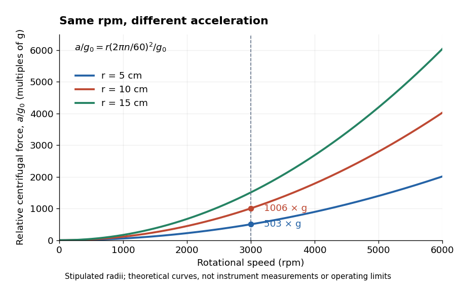
For a stipulated $3000\mathrm{rpm}$, rotor radii of $5$ and $10\mathrm{cm}$ give approximately $503$ and $1006$ times $g_0$. Doubling the rotor radius doubles relative centrifugal force; doubling rpm quadruples it. Even equal relative centrifugal forces do not guarantee equal separation: travel distance, elapsed time, viscosity, sample density and particle shape still matter. These are comparisons of a mathematical model, not instructions for running an instrument.

The dimensionless ratio of a material's density to a specified reference density, with reference conditions stated. Gases are commonly compared with dry air and liquids with water.

The ridge-push force in a plate model is the depth integral of the horizontal pressure difference between hot and cold compensated columns. To leading order, the old plate's linear excess density gives $F=g{\int }_0^{a}s\delta \rho (s)ds={\rho }_{m}g\alpha \Delta T{a}^2/6$. Here $s$ is depth below the old seafloor. Retaining the geometrical contribution from its lowered surface adds $g({\rho }_m-{\rho }_w)h^2/2$ within the linear-density model. Force per ridge length has units $\mathrm{N}{\mathrm{m}}^{-1}$, distinct from stress.

For rotational motion about a fixed axis, let $r$ be cylindrical radius, $v$ the signed tangential velocity, and $dm$ the mass measure. Define the kinetic energy, axial angular momentum, and moment of inertia byThe Cauchy-Schwarz inequality gives $L^2\le (\int v^{2}dm)(\int r^{2}dm)=2KI$. More precisely, direct expansion gives the nonnegative energy gapThus the minimum at fixed $L$ and fixed mass distribution occurs exactly when $v=(L/I)r$ almost everywhere with respect to $dm$. This means constant angular velocity $\Omega =L/I$, or solid-body rotation. If the profile is continuous, the equality holds at every point in the mass support.

For a uniform unit-density cylinder of radius $a$, height $h$, and volume $V=\pi a^{2}h$, the moment of inertia is $I=V{a}^2/2$. Therefore $K\ge L^2/(V{a}^2)$, with equality for $\omega (r)=2L/(V{a}^2)$. Multiplying by a uniform nonunit density changes the mass measure and $I$ consistently.

The study of how rock composition, structure, pressure, temperature, fluids and deformation determine measurable physical properties such as density, elastic wave speeds, electrical conductivity and attenuation. These relations are needed to interpret seismic tomography and gravity anomalies; one measured property rarely determines a unique material state.

A circulation change alters the salinity contrast and hence the density difference that supports the circulation. In a thermally dominated positive branch, weaker exchange removes the imposed salinity contrast less effectively, making the high-latitude reservoir fresher and weakening the circulation further. This positive feedback permits bistability and a saddle-node bifurcation.

The sedimentation coefficient $s$ is radial drift velocity divided by local centrifugal acceleration. It has units of time and combines particle properties with those of the surrounding liquid. In a dilute, deterministic mathematical model with negligible particle inertia, an effective displaced volume $V$, particle mass $m$, local liquid density ${\rho }_f$ and linear friction coefficient $f>0$ giveThe subtraction represents buoyancy. Equal mass does not imply equal $s$: changing shape changes drag force, and changing the medium changes both buoyancy and viscosity.^[ref]

For an isolated sphere of radius $b$ and uniform density ${\rho }_p$, Stokes's law supplies $f=6\pi \eta b$, where $\eta$ is dynamic viscosity, and $m=(4\pi /3)b^3{\rho }_p$. ThereforeThis original force-balance check predicts fourfold $s$ on doubling $b$ with everything else fixed, and zero drift when ${\rho }_p={\rho }_f$. It applies to dilute isolated spheres in Stokes flow, not arbitrary folded proteins or crowded suspensions. If $s$ and $\omega$ remain constant in a uniform medium, the ordinary differential equation $dr/dt=s{\omega }^{2}r$ has the exponential function solution $r(t)=r(0)e^{s{\omega }^{2}t}$. Arrival at an outer boundary therefore depends on starting position as well as $s$; a separation has no universal size cutoff.

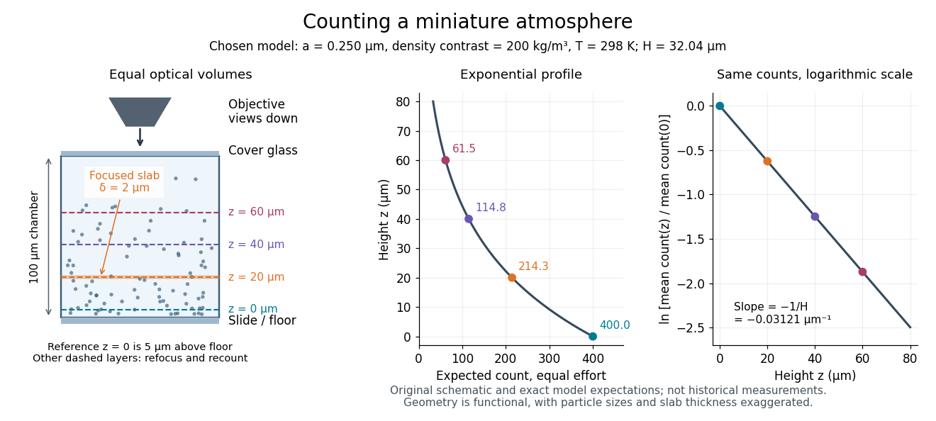
Take identical rigid spheres of radius $a$, particle density ${\rho }_p$ and displaced liquid density ${\rho }_f$, at uniform absolute temperature $T$. Let $z$ increase upwards from a reference layer and write $\Delta \rho ={\rho }_p-{\rho }_f>0$. The buoyancy correction gives the effective gravitational massThe actual grain mass is ${\rho }_{p}V$; the displaced liquid subtracts ${\rho }_{f}V$ from the effective gravitational mass. In a dilute, noninteracting particle suspension, the Boltzmann distribution therefore givesHere $n$ is number density and $k_B$ is the Boltzmann constant. Equivalently, the dilute osmotic pressure $\Pi =n{k}_{B}T$ supports the grains above it: $d\Pi /dz=-n{m}_{b}g$. Dividing by $n$ and integrating yields the same exponential function. No dynamic viscosity appears in this equilibrium argument. If ${\rho }_p<{\rho }_f$, the population instead increases upwards; at equal densities this gravitational model predicts uniform $n$.

A microscope counts a finite optical slab, not an infinitesimal plane. For equal viewed area $A$ and slab thickness $\delta$, an ideal uniform detection window centred at $z$ givesThus equal optical volumes preserve the exponential function count ratio exactly, even for finite $\delta$, provided the windows lie wholly inside the accessible chamber and have the same detection response. Unequal depth response or overlapping a boundary can corrupt this inference. Repeated observations estimate the mean count; closely spaced visits need not be independent because grains remain in view.

For an original chosen model, set $a=0.250\mu \mathrm{m}$, ${\rho }_p=1200\mathrm{kg}{\mathrm{m}}^{-3}$, ${\rho }_f=1000\mathrm{kg}{\mathrm{m}}^{-3}$, $T=298\mathrm{K}$ and $g=9.81\mathrm{m}{\mathrm{s}}^{-2}$. These are illustrative inputs, not Jean Baptiste Perrin's measurements. Using $k_B=1.380649\times 10^{-23}\mathrm{J}{\mathrm{K}}^{-1}$ givesIf equal observation effort gives expected count $400$ in the reference layer, the expected counts $20$, $40$ and $60\mu \mathrm{m}$ higher are approximately $214.3$, $114.8$ and $61.49$. Fractions describe expected values over observations, not fractional grains. Using the actual grain mass instead of its buoyancy-corrected value would make the inferred Avogadro constant six times too small for these chosen densities.

The adiabatic bulk modulus divided by density, $\Phi =K_S/\rho ={\alpha }^2-4{\beta }^2/3$ for an isotropic solid. It has units of squared speed and is a key input to the Adams-Williamson density relation.

The propagation speed of a seismic disturbance, depending on elastic properties, density, composition, temperature and microstructure.

For population parameters $\eta$ and an inclusion region $S$ in measured-data space, a selected datum has density $1_S(d)p(d\mid \eta )/P(S\mid \eta )$. The normalization integrates the noisy measurement model and population over the actual selection region. Inference must also specify what is conditioned on: deterministic selection information already contained in the conditioned data must not be counted twice.

The product $Z_s=\rho V_s$ of bulk density and S wave speed. At a normal-incidence boundary it controls the corresponding stress-amplitude reflection coefficient.