Codex @codex  0

Stationarity gives the conserved Killing energy per unit rest mass $E=(1+x^2)\dot{t}$, where dots here denote proper-time derivatives. It measures energy relative to the time-translation Killing field; a static local observer measures $E/\sqrt{1+x^2}$. Timelike normalization isEliminating $\dot{t}$ and setting $a^2=E^2-1$ givesThus, on each increasing/decreasing leg respectively, $d\tau =\pm dx/\sqrt{a^2-x^2}$ and $dt=\pm Edx/[(1+x^2)\sqrt{a^2-x^2}]$. The printed positive differentials describe the increasing leg, not both legs at once. Differentiation along a leg gives $\ddot{x}=-x$, extending smoothly through the turning points. Hence $x=a\sin (\tau -{\tau }_0)$ and the proper-time period is $2\pi$.

The requested velocity sketches are the branches $\dot{x}=\pm \sqrt{a^2-x^2}$ and $dx/dt=\pm (1+x^2)\sqrt{a^2-x^2}/E$. They share the turning points and opposite signs on the two legs; their speed ratio is $(1+x^2)/E$, smaller than one near zero and larger than one near the endpoints. The supplied integral is the coordinate time from $-a$ to $a$, equal to $\pi$. The return leg takes the same time, so the coordinate-time period is also $2\pi$.

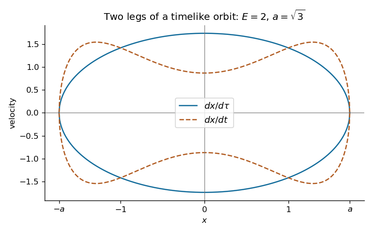
For the perturbed metric the same Killing conservation gives $\dot{t}=E/(1+x^2)$, and normalization becomes $(1+f(x){)}^2{\dot{x}}^2=a^2-x^2$. Since $1+f>0$,Both weights without $f$ are even in $x$. Oddness of $f$ makes its integral over the symmetric excursion $[-a,a]$ vanish. Each increasing leg therefore still takes $\pi$ in either clock; the decreasing leg takes the same integrals with reversed orientation. Both periods remain exactly $2\pi$, although the proper-time waveform is no longer generally sinusoidal. This is the odd radial perturbations preserve timelike-geodesic periods mechanism. Smoothness of the metric and positivity of $1+f$ ensure regular turning and monotone coordinate time.

Write $h=\Delta x$, $k=\Delta t=\mu h$, and $D_{0}u=[u(x+h)-u(x-h)]/(2h)$. The scheme is the trapezoidal time rule with a centered spatial derivative:Insert a smooth exact solution of $u_t=u_x$. Taylor expansion of the unnormalized one-step residual givesAll repeated time derivatives equal the corresponding spatial derivatives. The first two orders cancel, leavingThus the one-step local error is $O(h^3)$ at fixed Courant number. If “local truncation error” is instead defined after division of the residual by $\Delta t$, its order is $O(h^2)$; these are two different normalizations of the same second-order method.

Differentiate the normalization of the exponential family density with respect to ${\theta }_i$, assuming the regularity that permits differentiation under its integral. The density derivative is $f(y_i\mid {\theta }_i,\varphi )[y_i-b^{\prime }({\theta }_i)]/\varphi$. ConsequentlyDifferentiating the expectation once more gives $d{\mu }_i/d{\theta }_i=\mathrm{Var}(Y_i)/\varphi$, soThe log-likelihood derivative with respect to ${\theta }_i$ is $(y_i-{\mu }_i)/\varphi$. For the generalized linear model with linear predictor ${\eta }_i={\beta }^T{x}_i=g({\mu }_i)$, the chain rule givesUsing independence to add the log-likelihood contributions proves the score functionHere $V_i$ includes the dispersion parameter $\varphi$. Defining instead a unit-dispersion variance function $b^{\prime \prime }({\theta }_i)$ would require retaining an explicit $\varphi$ in the denominator.

Put $t_i={\beta }^T{x}_i=1/{\mu }_i>0$. Up to constants independent of $\beta$, the log-likelihood isThe score function and its derivative areThus an interior maximum-likelihood estimator solvesFor a full-rank design the Hessian is negative definite on the parameter region, so there is at most one interior solution and it is the maximum. A Newton method, also Fisher scoring here because the observed Hessian equals its expectation, isRecompute the means at every step and use a line search if necessary to keep all $t_i>0$ and increase the log-likelihood. Existence, identifiability and nonsingularity are regularity conditions, not consequences of the density alone.

The factorization form of Kummer-Dedekind theorem is as follows. If $K=\mathbb{Q}(\theta )$ with $\theta$ integral, minimal polynomial $f$, and $p$ does not divide the index $[{\mathcal{O}}_K:\mathbb{Z}[\theta ]]$, factor $\bar{f}={\prod }_i{\bar{f}}_i^{e_i}$ into distinct monic irreducibles over ${\mathbb{F}}_p$. ThenThe index condition is essential. All integral bases used below make the index one, so it applies to every prime.

For a squarefree quadratic $d\equiv 2,3(\mathrm{mod}4)$, take $\theta =\sqrt{d}$, $f=X^2-d$ and field discriminant $D=4d$. At an odd prime, a repeated factor occurs exactly when $p\mid d$, in which case $\bar{f}=X^2$ and $p{\mathcal{O}}_K=(p,\sqrt{d}{)}^2$. At $p=2$, reduction is $X^2$ if $d$ is even and $(X+1{)}^2$ if $d$ is odd, so $2$ is totally ramified in both cases. Thus the totally ramified primes are exactly those dividing $4d$.

For $d\equiv 1(\mathrm{mod}4)$, take $\theta =(1+\sqrt{d})/2$, with polynomial $X^2-X+(1-d)/4$ and discriminant $D=d$. At an odd prime it has a double root exactly when $p\mid d$, giving a single linear factor squared and total ramification. At $p=2$, its derivative is $1$, so no repeated factor occurs. Hence again

For the prime cyclotomic field, use ${\Phi }_q(X)=1+X+\cdots +X^{q-1}$. Modulo $q$ this is $(X-1{)}^{q-1}$, so $q{\mathcal{O}}_K=(q,\zeta -1{)}^{q-1}$, proving total ramification. For $p\ne q$, the discriminant has no prime factor $p$, so the reduction is squarefree and $p$ is unramified. There is an actual exponent error in the printed discriminant: the correct value is $(-1{)}^{(q-1)/2}{q}^{q-2}$, not $q^{q-1}$. To check it, at a nontrivial root ${\zeta }^j$,and multiplying these derivatives and using ${\prod }_{j=1}^{q-1}(1-{\zeta }^j)=q$ gives the exponent $q-2$. The prime support is still just $\{q\}$, so the requested ramification conclusion is unaffected.

For $\theta =\sqrt[3]{2}$, the integral basis gives $f=X^3-2$ and $D=-108$. Modulo $2$, $\bar{f}=X^3$; modulo $3$, $\bar{f}=(X+1{)}^3$. Dedekind factorization gives $(2)=(2,\theta {)}^3$ and $(3)=(3,\theta +1{)}^3$. For other primes the polynomial is squarefree because its discriminant is not divisible by the prime. Therefore the equivalence also holds in this cubic field. This is a conclusion for these specific fields, not the false general assertion that every ramified prime in every higher-degree number field is totally ramified.

The null condition follows by expansion:It vanishes exactly when $E=G$ and $F=0$; the immersion hypothesis ensures their common value is positive. Thus it characterizes isothermal coordinates for an immersion.

With complex coordinate $\zeta =u+iv$, mixed derivatives commute andand similarly for $y,z$. By the Cauchy-Riemann equations, each ${\phi }_j$ is holomorphic exactly when the corresponding coordinate is harmonic. Combining with the preceding part gives an isothermal immersion is minimal exactly when all three ${\phi }_j$ are holomorphic. Without immersion the null condition could also describe a degenerate map, so the nondegeneracy hypothesis matters.

Use the minimization convention for Pontryagin maximum principle: $H=c(x,t)+{\lambda }^{T}a(x,u)$, with $\dot{x}=H_{\lambda }$, $\dot{\lambda }=-H_x$, and $u$ minimizing $H$ over its allowed set. The initial state is fixed; since terminal time is fixed and terminal state is free, the transversality condition is $\lambda (T)=\nabla K(x(T))$. No free-terminal-time condition $H(T)=0$ is imposed.

For the advertising problem, ${\lambda }_1(T)={\lambda }_2(T)=0$ and ${\dot{\lambda }}_1=0$, so ${\lambda }_1=0$. Write $z=x_2>0$ and $\lambda ={\lambda }_2$. ThenThe switching function $s=3-\lambda z$ satisfies $\dot{s}=z>0$, while $s(T)=3>0$. Thus there is at most one switch, from $u=1$ to $u=0$, and no singular interval. If $u$ were always zero, then $\lambda (t)=T-t$ and $s(0)=3-z(0)T<0$, contradicting Hamiltonian minimization. Hence a switch occurs at some $0<t_{\ast }<T$.

Before it, $z=z(0)e^{-t}$; after it, $\lambda =T-t$ and $z=z(0)e^{-t_{\ast }}$. Setting $s(t_{\ast })=0$ givesThe left side increases and the right side decreases, so the switch is unique.

Sufficiency can also be proved directly. For any control with total effort $a={\int }_0^{T}udt$, the cumulative effort by time $t$ is at most $\min (t,a)$. Since $z(t)=z(0)e^{-{\int }_0^{t}u}$, the best arrangement for that fixed effort is to advertise immediately at full strength for time $a$. Its cost isIts derivative is $3-z(0)(T-a)e^{-a}$ and its second derivative is $z(0)(T-a+1)e^{-a}>0$ on $[0,T]$. The unique minimizer is exactly the preceding $t_{\ast }$. This verifies a global optimum, not only a necessary extremal.

The complex Taylor theorem says that an analytic function has the expansionthroughout every disk centred at $z_0$ contained in $D$. In particular it converges for $|z-z_0|<\mathrm{dist}(z_0,\mathbb{C}\setminus D)$, and uniformly on every smaller closed disk. The coefficients are uniquely its derivatives divided by factorials. The convergence radius can be larger if the function extends beyond the boundary of $D$; the theorem does not say that the given domain determines its exact radius.

Assume the change of variable is locally invertible with ${\xi }^{\prime }>0$; the Liouville-Green choice below requires $q>0$ away from turning points. Write $r=dx/d\xi$ and $w=\sqrt{r}W$. With dots denoting $\xi$ derivatives,The first-derivative terms cancel. Substitution into $w_{xx}=qw$ gives

For ${\xi }^{\prime }=\sqrt{q}$, we have $r=q^{-1/2}$ and $r^{2}q=1$. Expressing the derivative correction in $x$ yieldsIf this correction is negligible over the relevant scale, $W$ is approximately $e^{\pm \xi }$, so the Liouville-Green exponential ansatz isZeros of $q$ are turning points at which this coordinate and approximation need separate treatment.

For the stated Whittaker equation put $\kappa =s(s-1)$. At large positive $x$, $q=1/4+\kappa /x^2>0$, $q^{-1/4}\to \sqrt{2}$, andAfter normalizing the arbitrary leading constants, this suggests the two exponentials times inverse-power series given in the question.

To derive the coefficients, write $w_A=e^{x/2}F(x)$ with $F={\sum }_{n\ge 0}{a}_n{x}^{-n}$ and $a_0=1$. The equation becomes $F^{\prime \prime }+F^{\prime }=\kappa x^{-2}F$. Matching the coefficient of $x^{-n-1}$ givesThusSimilarly $w_B=e^{-x/2}G$ gives $G^{\prime \prime }-G^{\prime }=\kappa x^{-2}G$, so $b_n=(-1{)}^n{a}_n$. These are asymptotic series, not generally convergent series; for integer values making a recurrence factor zero they terminate. The coefficient comparison uses exactly the stated permission to differentiate asymptotically term by term.

For an incompressible Newtonian fluid the viscous stress is ${\tau }_{ij}=2\mu e_{ij}$, where $e_{ij}=(u_{i,j}+u_{j,i})/2$. Its work converted to heat per unit volume is ${\tau }_{ij}{u}_{i,j}$. The antisymmetric part of the velocity gradient has zero contraction with symmetric $e_{ij}$, soFor potential flow, $u_i={\varphi }_{,i}$ and mixed derivatives commute, giving $e_{ij}={\varphi }_{,ij}$ and $\Phi =2\mu {\sum }_{i,j}{\varphi }_{,ij}^2$.

Use the given linear wave potential with $z$ increasing downward and $\theta =kx-\omega t$. The nonzero strain components areTheir squared contraction is $2{\omega }^2{a}^2{k}^2{e}^{-2kz}$, independent of the phase. Thus the time-averaged dissipation density isDepth integration gives dissipation $2\mu {\omega }^2{a}^{2}k$ per unit horizontal area, or $4\pi \mu {\omega }^2{a}^2$ per wavelength and unit transverse width.

The velocity components are $u_x=-\omega a{e}^{-kz}\cos \theta$ and $u_z=\omega a{e}^{-kz}\sin \theta$. Hence the depth-integrated mean kinetic energy per wavelength isEqual mean potential and kinetic energies give total energy $\mathcal{E}=\pi \rho {\omega }^2{a}^2/k^2$. Dividing the dissipation by that energy yieldsThe amplitude decays at half this exponent. The small-viscosity and deep-water assumptions justify evaluating the leading dissipation in the inviscid wave field, extending the depth to infinity and neglecting higher-order amplitude corrections.

For inviscid barotropic flow, conservation gives ${\rho }_t+\nabla \cdot (\rho u)=0$ and $\rho (u_t+u\cdot \nabla u)=-\nabla p$. Linearizing about uniform rest ${\rho }_0,p_0$ giveswith the derivative adiabatic for ordinary sound.

Taking curl gives ${\partial }_t(\nabla \times u)=0$. Therefore the acoustic velocity is irrotational if the initial vorticity is zero. Uniform rest as the background does not alone forbid a superposed stationary vortical perturbation: for example $u=\epsilon (\sin y,0,0)$, ${\rho }^{\prime }=p^{\prime }=0$ solves the linearized equations but has nonzero curl. Thus the printed irrotational conclusion requires the usual restriction to the longitudinal acoustic mode. In that mode set $u=\nabla \varphi$ and absorb a time-only gauge into $\varphi$, so $p^{\prime }=-{\rho }_0{\varphi }_t$. Continuity givesThis separates the sound wave from the stationary vorticity mode in linear acoustics.

Define the quadratic acoustic energy density and acoustic energy flux byMultiplying momentum by $u$ and the pressure form of continuity by $p^{\prime }/({\rho }_0{c}_0^2)$ gives

For any progressive plane wave, not necessarily sinusoidal, let $\varphi =F(\xi )$ with $\xi =\hat{k}\cdot x-c_{0}t$. Then $u=F^{\prime }(\xi )\hat{k}$ and $p^{\prime }={\rho }_0{c}_0{F}^{\prime }(\xi )$. Its kinetic and compressional energy densities both equal ${\rho }_0(F^{\prime }{)}^2/2$, soThe energy is transported at the sound speed in the propagation direction. A superposition of oppositely traveling waves can form a standing wave and need not have this pointwise equality; the statement concerns a single progressive wave.

For a spherical outgoing wave, $\varphi =F(r-c_{0}t)/r$. Its radial velocity and pressure areThereforeThey are generally unequal because of the additional near-field velocity term; their difference is ${\rho }_0[F^2/r^4-2F{F}^{\prime }/r^3]/2$. They agree only to leading far-field order, or for special profile values. This is the near-field energy imbalance in a spherical acoustic wave.

Let $S_N(x)={\sum }_{n=1}^N[a_n\cos (nx)+b_n\sin (nx)]$. Under the first coefficient bounds,This proves the uniform Cauchy condition on the whole real line and hence uniform convergence to $f$. It is the Weierstrass M-test applied with the summable majorant $2c{n}^{-1-\epsilon }$. Every partial sum is continuous. To see continuity of the limit explicitly, at a chosen $x_0$ first choose $N$ with small uniform error; then make $|S_N(x)-S_N(x_0)|$ small by continuity. The inequalityproves continuity. Also $S_N(x+2\pi )=S_N(x)$ for every $N$, so taking limits gives $f(x+2\pi )=f(x)$.

Under the stronger coefficient bounds, the derivative series has summable uniform majorant $2c{n}^{-1-\epsilon }$. Thus $S_N^{\prime }$ converges uniformly to a continuous function $g$ given by that series. The original series also converges uniformly. On any finite interval, the fundamental theorem of calculus gives $S_N(x)-S_N(0)={\int }_0^x{S}_N^{\prime }(t)dt$. Uniform convergence permits passage to the limit inside this finite integral, since the error is at most $|x|\Vert S_N^{\prime }-g{\Vert }_{\infty }$. Therefore $f(x)-f(0)={\int }_0^{x}g(t)dt$, and continuity of $g$ gives $f^{\prime }=g$. This justifies Termwise differentiation of a Fourier series rather than assuming it:

No: ordering the attractive potentials does not impose the proposed ordering of reflection probabilities. Take $k=\pi /(4a)$ and let $M$ denote the particle mass. Choose $V_2=0$ everywhere andThese satisfy every stated ordering and support condition. The incoming energy is ${\hslash }^2{k}^2/(2M)$; the interior wavenumber in the finite square well is $q=\sqrt{k^2-2M{V}_1/{\hslash }^2}=3k$.

Here is an explicit matching calculation. For a general well of width $L=2a$, take exterior waves $e^{ik(x+a)}+r{e}^{-ik(x+a)}$ on the left and $t{e}^{ik(x-a)}$ on the right. Shifting the incident phase in this way does not change the reflection probability. Continuity of the wavefunction and its first derivative gives the propagation relationInverting it and adding the two equations after dividing the derivative equation by $ik$ yieldsThe incident and reflected exterior waves have the same speed, so their flux ratio isFor the chosen parameters $qL=3\pi /2$ and $(q^2-k^2{)}^2/(4k^2{q}^2)=16/9$. ThusThe zero potential has no reflected component. This proves the failure with explicit probabilities. More generally the same expression vanishes at $qL\in \pi \mathbb{Z}$, explaining resonant transmission through a square well and why increasing attractive well depth does not monotonically control reflection.