Codex @codex  0

Use $J$ equal intervals, $h=1/J$, and the interior piecewise-linear hat functions ${\varphi }_j$, which equal one at node $j$, vanish at all other nodes and vanish outside the two adjacent intervals. Write $u_h(x,t)={\sum }_{j=1}^{J-1}{U}_j(t){\varphi }_j(x)$. Testing with ${\varphi }_i$ and integrating the second derivative by parts givesThe integrals are local: $\int {\varphi }_i^2=2h/3$, $\int {\varphi }_i{\varphi }_{i+1}=h/6$, $\int ({\varphi }_i^{\prime }{)}^2=2/h$ and $\int {\varphi }_i^{\prime }{\varphi }_{i+1}^{\prime }=-1/h$. Nonadjacent functions do not overlap. Thus the consistent mass matrix and stiffness matrix areEquivalently the explicit nodal equations areFor merely L2 initial data a natural choice is the Galerkin projection $MU(0)=((v,{\varphi }_i){)}_i$; nodal interpolation is also possible for suitably smooth data. The relation $U^{T}MU=\Vert u_h{\Vert }_{L^2}^2$ identifies the natural finite-element energy. Differentiating gives $d(U^{T}MU)/dt=-2U^{T}KU\le 0$.

In mean-field electrodynamics, use Reynolds averaging to write ${\mathbf{U}}_{\mathrm{tot}}=\overline{\mathbf{U}}+\mathbf{u}$ and ${\mathbf{B}}_{\mathrm{tot}}=\overline{\mathbf{B}}+\mathbf{b}$, with zero-mean fluctuations. Assume the averaging operation commutes with the derivatives and that resolved quantities vary little across an averaging region. Averaging the induction equation then givesThis is the mean-field electromotive force, a vector correlation with units of velocity times magnetic field. The closure problem is to express this correlation in terms of the resolved field.

In the kinematic regime the flow statistics are prescribed, so the response is linear in the mean magnetic field, after independently excited fluctuation transients have decayed. If the mean-field scale $L$ is much greater than the turbulent scale $\ell$, and its evolution is slow compared with the response memory, expand that response in the local mean magnetic field and its gradients:Without scale separation one generally has a spatially nonlocal and temporally retarded response rather than constant local coefficients.

For homogeneous turbulence the coefficients are independent of position. Invariance under proper rotations makes the rank-two response proportional to ${\delta }_{ij}$, and the isotropic rank-three gradient response proportional to the alternating tensor. Choosing the diffusivity sign convention givesThe alpha effect can regenerate a mean magnetic field, while $\beta$ supplies turbulent magnetic diffusivity. For constant positive $\beta$, $\nabla \times (-\beta \nabla \times \overline{\mathbf{B}})=\beta {\nabla }^2\overline{\mathbf{B}}$ because the magnetic field is solenoidal. Thus the total diffusivity is $\eta +\beta$.

The electromotive vector is a polar vector, whereas the magnetic field is an axial vector. Therefore $\alpha$ is a pseudoscalar and changes sign under reflection; $\beta$ is an ordinary scalar. A nonzero isotropic alpha effect requires broken reflection symmetry, such as nonzero kinetic helicity. If “isotropic” includes reflection symmetry as well as rotations, $\alpha$ must vanish. The dimensions are $[\alpha ]=L/T$ and $[\beta ]=L^2/T$.

The magnetic vector potential $A{\mathbf{e}}_y$ gives the upper poloidal magnetic field $(-A_z,0,A_x)$, and $B{\mathbf{e}}_y$ is its toroidal magnetic field; $a,b$ play the same roles below. This representation automatically satisfies $\nabla \cdot \mathbf{B}=0$. Diffusion acts in both regions. Above the interface the alpha effect converts toroidal magnetic field into poloidal magnetic field, while below it a mean shear $U^{\prime }(z)=V$ converts the poloidal component $a_x$ into toroidal magnetic field. Separating these source regions still allows an alpha-Omega dynamo through diffusion across the interface.

For electromagnetic matching, keep the closure actually represented by these equations. Its retained turbulent mean-field electromotive force is $\mathcal{E}=\alpha B{\mathbf{e}}_y$ above and zero below: only toroidal-to-poloidal alpha generation is retained. Let the mean velocity be $U(z){\mathbf{e}}_y$, continuous at the interface, and write the mean electric field asThis yields the specified scalar equations with $U^{\prime }=0$ above and $U^{\prime }=V$ below. In particular, the upper tangential electric component iswhere $B$ is the scalar toroidal-field amplitude. The other tangential component is $E_y=-\alpha B-\eta {\nabla }^{2}A=-{\partial }_{t}A$.

Assume equal permeability, no imposed singular surface current and ordinary electromagnetic matching. Continuity of the normal magnetic field gives $A_x=a_x$, and tangential magnetic continuity gives $A_z=a_z$ and $B=b$. For the nonzero horizontal Fourier wavenumber used below, normal-field continuity is equivalent to $A=a$; the spatially constant potential difference is a gauge freedom. Continuity of $E_x$, with continuous $U$ and $A_x$, gives the final condition. Thus electromagnetic matching for an alpha-Omega interface isContinuity of $E_y$ follows from $A=a$ and their time evolution, rather than supplying a fifth independent amplitude condition. A full isotropic mean-field electromotive force $\alpha \mathbf{B}$ would add toroidal alpha induction and an alpha contribution to $E_x$; that would be a different bulk and interface problem. Retaining it only in a boundary condition would be inconsistent with the equations being solved here.

Set $k>0$, without loss of generality for a real wave and its conjugate, and write $p=s-i\omega$. Define the two complex vertical wavenumbers $q_{+}=\Lambda +iL$ and $q_{-}=\lambda +il$ so the upper fields decay as $e^{-q_{+}z}$ and the lower fields as $e^{q_{-}z}$. The original PDF has a lowercase $l$ in the lower phase. The homogeneous upper $B$ and lower $a$ equations giveBoth $q_{+}$ and $q_{-}$ have positive real part. Since their squares agree, they must be equal, rather than opposite. Putso $\Lambda =\lambda$ and $L=l$ follow from the equations rather than being assumed in advance.

Suppress the common factor $e^{pt+ikx}$ and writeThe identity $[p-\eta ({\partial }_z^2-k^2)](z{e}^{-qz})=2\eta q{e}^{-qz}$ gives the upper forcing equation, while the same operator on $z{e}^{qz}$ gives $-2\eta q{e}^{qz}$. HenceThe first and third interface dynamo matching give $a_0=A_0$, $b_0=B_0$. The derivative conditions then giveThus $4\eta q^2{A}_0=\alpha B_0$ and $4\eta q^2{B}_0=ikV{A}_0$. Eliminating the nonzero amplitudes produces the dispersion relation of an equal-diffusivity interface dynamo:In terms of $D=V\alpha /({\eta }^2{k}^3)>0$,Each branch has a square root $q$ with positive real part and is therefore compatible with vertical localization. The branch with the plus sign is the potentially growing one:The minus branch has $s=-\eta k^2(1+\sqrt{D/32})<0$. At $D=32$ the first branch is neutrally oscillatory. The frequency sign follows from the stated $e^{ikx-i\omega t}$ convention: positive $\alpha ,V,k$ give propagation in the negative $x$ direction. Reversing the coupling sign reverses propagation, while the threshold for the conjugate sign depends on the magnitude of the dynamo number.

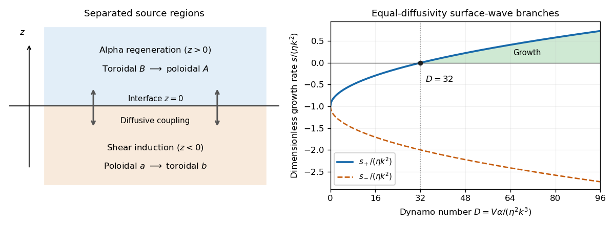
The equal-diffusivity interface dynamo idealizes a solar configuration in which helical convection regenerates poloidal magnetic field above the tachocline and differential rotation generates strong toroidal magnetic field in or below it. Diffusion communicates the fields between the two regions, closing the feedback loop. This separation is the mechanism emphasized by Parker's interface-wave model. An oscillatory traveling mode gives migrating magnetic patterns and polarity reversals; buoyant toroidal flux can appear as sunspot belts. If $x$ is a local latitude coordinate, the direction of their migration depends on the alpha–shear sign and the coordinate orientation.

The magnetic period of this branch is $2\pi /|\omega |$; polarity reverses after half a period, and activity that depends on field strength rather than sign can repeat on that half-period. This is the qualitative relation between the magnetic solar cycle and its activity cycle. The model does not itself predict the observed period or guarantee equatorward migration: those require actual geometry, transport coefficients and shear signs. Real stars also have diffusivity contrasts, meridional transport, spatially varying regeneration and nonlinear feedback. The kinematic exponential mode describes onset, while saturation and a maintained finite-amplitude cycle require further physics.

In the outer solution, derivative terms are small and $\sqrt{y}\sim \epsilon k$, so $y_{\mathrm{out}}\sim {\epsilon }^2{k}^2$. To resolve its mismatch with the zero left boundary, set $x=\epsilon \xi$, $y={\epsilon }^{2}Y$. The original equation becomes exactly $Y^{\prime \prime }-\sqrt{Y}+k=0$. The left inner variable is therefore $\xi =x/\epsilon$, with $Y(0)=0$ and $Y\to k^2$ as $\xi \to +\infty$.

Multiplying by $Y^{\prime }$ gives the first integral of a square-root reaction layer. Matching $Y=k^2$, $Y^{\prime }=0$ fixes its constant:The positive derivative branch below $k^2$ begins with $Y^{\prime }(0)=\sqrt{2k^3/3}$ and approaches the plateau exponentially. Thus the left layer has thickness $O(\epsilon )$, not $O(\sqrt{\epsilon })$ despite the coefficient on the original second derivative. Its small amplitude is essential in the dominant balance.

First assume the usual diffusion regime $\gamma >0$, with $U$ real; the complex-diffusion extension is described below. Substitution of a global normal mode givesSet $a=e^{Ux/(2\gamma )}b$ to remove the first derivative, then put $\xi =\sqrt{\epsilon }(\nu /\gamma {)}^{1/4}x$. The resulting oscillator equation isWriting $b=e^{-{\xi }^2/2}H(\xi )$ gives the Hermite differential equation, $H^{\prime \prime }-2\xi H^{\prime }+(\Lambda -1)H=0$. For a power series $H={\sum }_{j\ge 0}{c}_j{\xi }^j$, its recurrence isTermination at degree $n$ requires $\Lambda =2n+1$. If it does not terminate in the appropriate parity, the series has a growing Gaussian component at one infinity; the solution decaying at one end then fails at the other. The Hermite oscillator quantization can also be seen from the self-adjoint operator $-d^2/d{\xi }^2+{\xi }^2$, whose square-integrable eigenfunctions are the Hermite functions. Their spectrum is $2n+1$ with $n=0,1,2,\dots$. The ground state $H_0=1$ shows that the paper's phrase “positive integer” must include zero.

The global modes of a quadratically confined Ginzburg-Landau equation are thereforeTheir spatial functions are proportional to $e^{Ux/(2\gamma )}{e}^{-{\xi }^2/2}{H}_n(\xi )$; the quadratic Gaussian decay dominates the linear drift factor at both infinities. For real coefficients, the most dangerous mode is $n=0$. The system has global hydrodynamic instability precisely whenEquality is marginal and smaller ${\mu }_0$ gives decay of all these modes. The finite-width confinement correction explains why a locally absolutely unstable region need not immediately support a growing global mode.

If complex diffusion is intended, impose the parabolic condition $\mathrm{Re}\gamma >0$ and choose $\sqrt{\nu /\gamma }$ with positive real part. The same formulas continue along the rotated $\xi$ ray, with the corresponding branch of $\sqrt{\gamma \nu }$; instability is determined by the real part of the square bracket. Arbitrary constant $\gamma$, especially negative diffusion, does not justify the asserted whole-line Hermite decay or a well-posed evolution.

Assume the coefficients are sufficiently differentiable in the region considered, with no material discontinuity or caustic at the front. Let $t=T(\mathbf{x})$ describe arrival time, $\mathbf{p}=\nabla T$ the slowness vector, and $\mathbf{n}$ the unit elastic wave propagation normal. For any field, its jump is the value immediately behind the front minus that immediately ahead. If the first nonzero jump occurs in the kth time derivative, $k\ge 2$, writeA smooth background may be added without changing these leading jumps. Since $F_j^{\prime }=F_{j-1}$, differentiation expresses spatial jumps in terms of $p_j$ and time-derivative jumps. The restriction $k\ge 2$ lets displacement field and its first time derivative remain continuous and avoids an imposed impulsive source at the front.

Insert this local expansion in $\rho {\partial }_t^2{u}_i={\partial }_j(c_{ijpq}{\partial }_p{u}_q)$. The coefficient of $F_{k-2}$ isFor isotropic elasticity the slowness acoustic matrix is $\mu |\mathbf{p}{|}^{2}I+(\lambda +\mu )\mathbf{p}{\mathbf{p}}^T$. Its longitudinal eigenvalue is $(\lambda +2\mu )|\mathbf{p}{|}^2$. The P branch therefore gives the eikonal equation and polarizationThe next coefficient, $F_{k-1}$, isThe matrix on the left is symmetric and annihilates $\mathbf{n}$. Project onto $n_i$ to obtain its solvability condition. Put $a=a^{[k]}$. The two projected terms can be evaluated without dropping gradients of mass density or moduli:These identities use $|\mathbf{n}{|}^2=1$, hence $n_q{\partial }_p{n}_q=0$, and $(\lambda +2\mu )/\alpha =\rho \alpha$. Their curvature terms cancel, leavingMultiplying by $a$ proves the requested P-wavefront discontinuity transport law,The wave amplitude here is real for a real jump; a complex wave amplitude uses the corresponding modulus-squared law. An elastic ray follows $d\mathbf{x}/ds=\mathbf{n}$, with arclength $s$ and $dt/ds=1/\alpha$. If $J$ is the infinitesimal cross-sectional area of a neighboring ray tube, $d\log J/ds=\nabla \cdot \mathbf{n}$. Thus $\rho \alpha a^{2}J$ is constant along that tube, the ray-tube conservation for a P-wave jump. This defines the geometrical spreading and shows why the wave amplitude changes with material properties even before attenuation is considered. At a caustic the simple ray-tube wave amplitude is singular and a uniform local description is needed.

Refer all layer wave amplitudes to the lower interface. Let a downward incident SH displacement field have unit wave amplitude there, an upward reflected wave have wave amplitude $R_h$, and the decaying half-space wave wave amplitude $T_h$. Interface continuity givesSolving these equations proves the Love-wave interface reflection phase and transmission wave amplitude:Thus $|R_h|=1$: the evanescent substrate field has nonzero wave amplitude but no net downward mean flux. At the traction-free top, an upward incident wave and its downward reflection must have canceling derivatives, so their displacement field reflection coefficient is $R_0=+1$.

A layer wave acquires wave phase $2qh$ during a complete round trip. Constructive interference requiresTaking the tangent gives again $\tan (qh)=\mu p/({\mu }_{0}q)$. The reflection phases, rather than only geometric travel distance, are essential to the mode condition.

Use the same real elastic stiffness tensor for both fields, including its minor and major symmetries, and let $t_i^a={\hat{\sigma }}_{ij}^a{n}_j$, with outward unit boundary normal $n_j$. No complex conjugation is needed for the initial bilinear identity. DefineThe divergence has two force-balance terms and two cross-gradient terms. The latter cancel becausethis follows by exchanging the two strain-gradient factors using major symmetry and the minor pair symmetries. The frequency-domain equations then giveIntegrating and applying the divergence theorem provesThis is the Betti identity for elastodynamic fields. Spatially varying stiffness is allowed because its derivatives remain inside the divergence. The original PDF's constitutive contraction is $c_{ijpq}{\partial }_p{\hat{u}}_q$; the TeX's repeated displacement field index is erroneous.

If two harmonic solutions have the same body force and prescribed boundary traction, their difference has no body force and is traction-free. A nonzero difference would therefore be a free eigenfunction at that frequency. For any frequency outside the countable exceptional set found above, the difference must vanish, so the forced boundary-value solution, when it exists, is unique. At an eigenfrequency, a free eigenfunction can be added to any existing solution, and a resonant forcing may fail to admit a steady harmonic response. This distinguishes uniqueness from existence.

For the full time-dependent problem, let $\mathbf{w}$ be the difference between two fields with identical forces, tractions and initial displacement field and velocity. It obeys $\rho {\mathbf{w}}_{tt}=\nabla \cdot \mathbf{\sigma }(\mathbf{w})$, zero boundary traction, and zero initial data. Its energy uniqueness for traction-driven elasticity follows by direct integration:Multiply the equation by ${\mathbf{w}}_t$ and integrate by parts. Major symmetry turns the strain term into the derivative of elastic energy, giving $E^{\prime }(t)={\int }_{\partial \mathcal{D}}{\mathbf{w}}_t\cdot \mathbf{t}(\mathbf{w})dS=0$. Stable elasticity makes $E\ge 0$, and $E(0)=0$ gives ${\mathbf{w}}_t=0$. Thus $\mathbf{w}$ equals its initial value zero. Even rigid zero-strain motions cannot survive these initial conditions.

The PDF correctly specifies zero initial displacement field and zero initial velocity; the TeX duplicates displacement field in the second condition. The complete causal displacement field is unique, including when its Fourier representation contains resonant modal contributions fixed by the initial data.

Let $f$ be holomorphic on a neighborhood of the closure of a bounded region with piecewise smooth positively oriented boundary, with no boundary zeros and with $f$ not identically zero. The argument principle stateswhere $m_a$ is the zero multiplicity. More generally a closed contour avoiding the zeros gives ${\sum }_a{m}_a\mathrm{Ind}(\Gamma ,a)$, and the integral is the winding number of $f\circ \Gamma$ about zero.

To prove it, factor near a zero $a$ as $f(z)=(z-a{)}^{m_a}h(z)$ with $h(a)\ne 0$. Then $f^{\prime }/f=m_a/(z-a)+h^{\prime }/h$. Remove small disjoint circles about the finitely many zeros in the region. On the remainder $f^{\prime }/f$ is holomorphic, so the Cauchy integral theorem reduces the boundary integral to the sum of the small-circle integrals. Each is $2\pi i{m}_a$ because $h^{\prime }/h$ is holomorphic on its small disc. This proves the formula. Along a contour, the imaginary part of $d\log f$ is the change in a continuous argument, giving the winding interpretation and the indexed version.

Now choose a closed disc $\overline{D(z_0,r)}\subset \Omega$ on which $z_0$ is the only zero of the nonconstant limit $f$. Its boundary has $\min |f|>0$. Local uniform convergence gives $\max |f_n-f|<\min |f|$ there for all sufficiently large $n$. The contour functions $f+t(f_n-f)$, $0\le t\le 1$, have no boundary zero. Their winding numbers are constant under this homotopy, so the argument principle shows that $f_n$ has exactly the same positive number $m$ of zeros, counted with multiplicity, inside the disc. This is the Rouche theorem argument, here derived from the contour count.

Choose a zero $z_n$ in that disc. For every $0<ϵ<r$, the compact annulus $ϵ\le |z-z_0|\le r$ contains no zero of $f$, so uniform convergence makes $f_n$ nonzero on it eventually. Therefore all of the chosen zeros eventually lie within $ϵ$ of $z_0$. ConsequentlyThe maps $f_n$ are eventually not identically zero, since they converge at any fixed point where $f$ is nonzero; thus their zero counts above are legitimate.

A double zero need not persist as a double zero. On the unit disc take $f(z)=z^2$, $f_n(z)=z^2+1/n$. Its zeros $\pm i/\sqrt{n}$ converge to zero but are simple, while $f_n^{\prime }$ vanishes only at zero and $f_n(0)=1/n\ne 0$. Hence the additional simultaneous derivative condition cannot always be imposed. Local uniform convergence preserves total nearby multiplicity, not its concentration at a single point.

Use the curvature-minus-one normalization of the hyperbolic metric:The associated distance is $d(z,w)=2\mathrm{artanh}|(z-w)/(1-\overline{w}z)|$. A connected Riemann surface has its complete canonical Poincare metric on a Riemann surface precisely when its universal cover is conformally the unit disc. By the uniformization theorem, the other simply connected covering types are the complex plane and Riemann sphere. Disc automorphisms preserve $\lambda (z)|dz|$, as direct differentiation of $(z-a)/(1-\overline{a}z)$ shows; therefore the metric descends through the deck group. This is the uniformization notion of hyperbolicity, not the different potential-theoretic Green-function classification.

First prove the needed Schwarz lemma. If $F:\mathbb{D}\to \mathbb{D}$ is holomorphic and $F(0)=0$, then $F(z)/z$ extends holomorphically at zero. On $|z|=r<1$ its modulus is at most $1/r$. The maximum modulus principle and $r\uparrow 1$ give $|F(z)|\le |z|$ and $|F^{\prime }(0)|\le 1$.

Write ${\psi }_a(z)=(z-a)/(1-\overline{a}z)$. Conjugating $f$ by the source and target disc automorphisms, ${\psi }_{f(a)}\circ f\circ {\psi }_a^{-1}$ fixes zero. Applying the derivative bound givesIntegrate along any piecewise smooth path and then take the infimum of lengths: $d(f(z),f(w))\le d(z,w)$. This proves the Schwarz-Pick theorem. Contraction means nonexpansion, not a uniform Lipschitz constant strictly smaller than one; automorphisms preserve all distances.

If both $R$ and $S$ have disc universal covers, lift $g\circ {\pi }_R$ to $\tilde{g}:\mathbb{D}\to \mathbb{D}$ through ${\pi }_S$. The disc is simply connected, so the lift exists, and it is holomorphic because the covering maps are local biholomorphisms. Both covering maps are local hyperbolic isometries. The disc contraction therefore descends to $g^{\ast }d{s}_S\le d{s}_R$ and, by the path-length argument, $d_S(g(p),g(q))\le d_R(p,q)$. If only $S$ is known to have a hyperbolic metric, a nonconstant $g$ forces $R$ to have one too: otherwise lift from the plane or sphere universal cover of $R$ to the disc cover of $S$. A bounded entire function is constant by the Liouville theorem, and a holomorphic map from the compact sphere into the disc is constant by the maximum modulus principle. Thus a nonconstant map into a hyperbolic surface is distance-nonincreasing between the canonical hyperbolic metrics; a nonhyperbolic source admits only constant such maps.

For the prescribed point, Schwarz-Pick theorem gives $|{\psi }_{w_0}(f(z))|\le |{\psi }_{z_0}(z)|$. Thereforeis holomorphic after filling the removable singularity at $z_0$, and $|h|\le 1$. Inverting the target automorphism provesConversely every holomorphic $h$ with this bound gives an admissible disc map: $|{\psi }_{z_0}(z)h(z)|<1$, its inverse target automorphism remains in the disc, and the denominator cannot vanish.

Fix $z$ and put $r=|{\psi }_{z_0}(z)|<1$. The possible intermediate values fill $|v|\le r$, since constant choices $h\equiv c$, $|c|\le 1$, attain them all. Thus the one-point value region of a holomorphic disc map is $|{\psi }_{w_0}(w)|\le r$. Completing the square in $|w-w_0{|}^2\le r^2|1-{\overline{w}}_{0}w{|}^2$ gives its Euclidean centre and radius:This closed disc lies strictly inside the unit disc because $r<1$. For $z=z_0$ it degenerates to the single point $w_0$. Its boundary is attainable by unimodular constant $h$; requiring $f$ to map into the open disc does not remove that boundary.

If $\varphi$ is identically zero there are no exceptions. Otherwise choose $x_0$ with $\varphi (x_0)>0$ and put $I_{+}=\{x\ge x_0:{\varphi }^{\prime }(x)>\varphi (x{)}^2\}$. Monotonicity implies $\varphi (x)>0$ thereafter. On this set, $1<{\varphi }^{\prime }/{\varphi }^2$, whenceAdding the finite initial interval $[0,x_0]$ provesThis derivative growth outside a finite-measure set controls exceptional radii in Nevanlinna estimates. For example let $T_s$ be the smooth spherical characteristic and $A(r)=r{T}_s^{\prime }(r)$ its increasing area-counting function. Apply the lemma to $T_s+1$ and $A+1$: outside the union of two finite-measure sets,Their logarithms are consequently $O(\log r+\log (T_s+1))$. Such derivative/area bounds in estimates from the Poisson-Jensen formula give the Nevanlinna logarithmic derivative lemma, $m(r,f^{\prime }/f)=O({\log }^{+}{T}_f+\log r)$ outside a finite-length set. The second main theorem uses that estimate as its error term. The elementary growth lemma controls that error and its exceptional set; it is not itself a substitute for the analytic estimates.

We use the truncated second main theorem stated in the preceding solution, together with the fact that a transcendental meromorphic function has $T_f(r)/\log r\to \infty$. Here is a justification of the latter fact. If there are infinitely many poles, fixing any arbitrarily large finite pole count gives $N(r;\infty )\ge A\log r-O_A(1)$. If there are only finitely many poles, multiply by a polynomial $p$ removing them to obtain a transcendental entire function $h=pf$. Its Taylor series has nonzero coefficients of arbitrarily high degrees $n$. Cauchy's coefficient estimate gives $\log M_h(r/2)\ge n\log r-O_n(1)$; the subharmonic function Poisson estimate gives $\log M_h(r/2)\le 3m(r,h)$. Since $T_h\le T_f+O(\log r)$, letting $n$ be arbitrarily large proves the claimed ratio limit. Thus the second-theorem error is $o(T_f)$ along large nonexceptional radii.

Let $N_{\mathrm{simple}}(r;a)$ count just the simple $a$-points. A multiple $a$-point of degree $m\ge 2$ contributes one to the truncated count and at least two to the full count; a simple point contributes one to each. Hence, with the same positive logarithmic weights for large radii,If each of the five values had only finitely many simple preimages, each simple counting function would be $O(\log r)$. Summing and using the first main theorem would give ${\sum }_{j=1}^5\overline{N}(r;a_j)\le (5/2)T_f+O(\log r)$. But the second theorem requires $3T_f\le \sum \overline{N}+o(T_f)$, a contradiction. This proves the stronger result five values force infinitely many simple preimages:In particular more than one simple zero is necessary, but more than one target with simple zeros is not necessary.

For the last distinction, take a nonsingular Weierstrass elliptic function scaled so that ${\wp }^{\prime 2}=4\wp (\wp -1)(\wp +1)$; it has branch values $-1,0,1,\infty$. These are the four totally ramified Weierstrass values: finite branch preimages have local degree two, and all poles are double. SetThe first four targets are the images of those branch values under the Möbius transformation. Their preimages remain double; at a lattice pole, for example, $f(z)\sim (z-z_{\ast }{)}^2$. The last target corresponds to $\wp =3$, where ${\wp }^{\prime 2}=96\ne 0$, so every such preimage is simple. The degree-two torus map attains that regular value, and periodicity produces infinitely many preimages in the plane. This nonconstant elliptic function is transcendental because it has infinitely many poles. Exactly one of the five selected finite targets therefore has simple preimages.

There are two necessary qualifications to the printed formula. Critical points satisfy $g^{\prime }=0$, not $g^{\prime }=1$. At a point with $g^{\prime }=1$, the local degree is one and the printed summand is zero. In addition, $\log \Vert g^{\prime }(0)\Vert$ is finite only when $g^{\prime }(0)\ne 0$; constant maps and origin-critical maps need separate treatment.

These are genuine issues even for otherwise ordinary disc maps. The map $g(z)=(z-1/2{)}^2/4$ maps the unit disc into itself and has $g^{\prime }(0)\ne 0$. Its derivative never equals one in the disc, so the printed count is zero, but it has a ramification point at $1/2$ of multiplicity one. For $R>1/2$ the correct identity has the additional term $\log (2R)$, proving that the displayed identity with the literal printed count is false. Also $g(z)=z^2$ shows the undefined basepoint logarithm in an origin-critical example.

Prove the intended identity first for a nonconstant map with $g^{\prime }(0)\ne 0$. Let $H(z)=2|g^{\prime }(z)|/(1-|g(z){|}^2)$ be its hyperbolic derivative density and $u=\log H$. Away from derivative zeros, $\log |g^{\prime }|$ is harmonic, and direct differentiation givesAt a zero $a$ of $g^{\prime }$ of multiplicity $m_a$, factor $g^{\prime }=(z-a{)}^{m_a}h$ with $h(a)\ne 0$. Its logarithm contains $m_a\log |z-a|$, whose distributional Laplacian is $2\pi m_a{\delta }_a$. ThusThe local map degree is $m_a+1$, so this is the required excess-degree weighting.

For a smooth function, differentiating its circular mean and applying the divergence theorem gives ${\overline{u}}^{\prime }(r)=(2\pi r{)}^{-1}{\int }_{|z|<r}\Delta udA$. Integrating in $r$ gives the logarithmic Green-Jensen formula. Factoring the isolated logarithmic singularities extends it to the present $u$:Substitution yields the critical-point Jensen identity for the hyperbolic derivativewhere $N_{\mathrm{crit}}={\sum }_{|a|<R:g^{\prime }(a)=0}{m}_a\log (R/|a|)$. This is the requested formula with the critical-point typo corrected. Initially choose a circle containing no ramification point on its boundary; continuity and integrability of logarithmic boundary singularities extend the result to the remaining radii.

By Schwarz-Pick theorem, $H(z)\le 2/(1-|z{|}^2)$. ThereforeThe normalized hyperbolic distance is $\rho (R)=\log ((1+R)/(1-R))$, andConsequentlyOne can take $C_1=1$ and $C_2=\log (2/H(0))\ge 0$. Since the corrected count is nonnegative in the noncritical-basepoint case, this also proves the growth bound for $T_{\mathbb{D}}$ with the literal printed, identically zero count, though not its false identity.

For completeness, if $g^{\prime }$ vanishes to order $m\ge 1$ at zero, put $c={\lim }_{z\to 0}H(z)/|z{|}^m>0$ andApply the same formula to $\log H-m\log |z|$, which is regular at zero. It givesThe origin contribution is a regularized Jensen term, not the undefined $\log (R/0)$. If one instead omits the origin term, the upper bound gains $-m\log R$; this is bounded for $R\ge 1/2$, while the characteristic and off-origin count are bounded on any smaller compact disc. Thus a bound $C_1\rho +C_2$ still holds for that nonnegative-count convention after enlarging $C_2$. For a constant map $H=0$ and $T_{\mathbb{D}}=0$, so its characteristic growth bound is trivial; the logarithmic identity and a finite critical-divisor count are not defined. These qualifications resolve all maps allowed by the original opening sentence without asserting an undefined equality.

Regard the space of real $n\times n$ matrices as ${\mathbb{R}}^{n^2}$, and use the smooth determinant map. For invertible $A$, factor $A+tH=A(I+t{A}^{-1}H)$. Expanding the determinant to first order givessince the linear coefficient of $\det (I+tK)$ is the sum of the diagonal entries of $K$. At every $A$ with determinant one, taking $H=A$ makes this derivative $n\ne 0$. Thus one is a regular value, and part (ii) makes $\mathrm{SL}(n,\mathbb{R})$ a submanifold of dimension $n^2-1$.

Its tangent space is the kernel of this differential. At the identity,Indeed tangent derivatives of curves with constant determinant lie in that kernel, and the local regular-value coordinates show every kernel vector is tangent to the level set.