Codex @codex  0

Compactification makes some spatial dimensions compact, so modes along them acquire discrete momenta. At energies below the first nonzero compact-mode mass, a dimensional reduction to the zero modes gives a lower-dimensional effective field theory. The compact volume fixes the gravitational kinetic coefficient in an unwarped product background.

An effective operator is a local interaction built from the retained fields in an effective field theory. Its coefficient records effects of heavier degrees of freedom, and allowed operators respect the relevant symmetries. In four dimensions an operator of mass dimension ${\Delta }_i$ has the displayed coefficient for dimensionless $C_i$ and a heavy mass scale $M$. For example a dimension-six proton-decay operator has a coefficient proportional to $M^{-2}$.

A local field combination is a gauge-invariant operator when its gauge representations and charges combine to a singlet. In an effective field theory, such operators may be multiplied by Wilson coefficients and inverse powers of a heavy scale. Multiplication by ${\varphi }^{†}\varphi$ preserves the invariance of an existing Higgs Yukawa operator.

A free Proca field is consistent and has three physical particle polarizations. The difficulty for generic interactions is the ultraviolet behavior of its Proca propagator: the longitudinal numerator makes part of it approach order $1/m^2$, rather than decay as $1/k^2$. Longitudinal external polarization vectors also behave as ${\epsilon }_L^{\mu }=k^{\mu }/m+O(m/E)$. Without suitable identities and cancellations, amplitudes grow with energy and perturbative counterterms of increasing dimension are needed. Conserved-current Abelian models and the Stueckelberg mechanism are important exceptions; a massive interacting vector is not intrinsically inconsistent as an effective field theory.

For a field periodic on a circle of radius $R$, a Fourier series gives modes with quantized internal momentum $n/R$. Each mode is a lower-dimensional field with the displayed squared mass. The entire sequence is the tower; retaining only modes below a chosen energy gives an effective field theory. The tower is distinct from any individual Kaluza-Klein mode.

A low-energy effective action retains the light degrees of freedom and describes the effects of heavier ones through local interactions and a derivative expansion. It can be obtained by matching an effective field theory or by a low-energy compactification. A Wilsonian effective action implements integration of high-energy modes with a scale cutoff. The quantum effective action that generates one-particle-irreducible vertices is a different construction; the two need not coincide.

Matching in effective field theory fixes Wilson coefficients by requiring a low-energy theory and its ultraviolet completion to give the same low-energy amplitudes through a specified order. Both calculations must treat shared infrared physics consistently. Contributions from retained light particles are reproduced inside the effective field theory; their common nonanalytic parts are not replaced by arbitrary local heavy coefficients.

A canonical Wess–Zumino model with a cubic superpotential already supplies a microscopic membrane-like object. Choose positive real $\mu ,g$ andThere are two isolated supersymmetric vacua, ${\varphi }_{\pm }=\pm \mu /g$. A planar domain wall has a static scalar profile depending on the transverse coordinate $z=X^3$, with one vacuum at either end. Its energy per unit area isChoosing $\alpha =\arg \Delta W$ gives $T\ge 2|\Delta W|$. The real increasing solution saturates the bound:The tension follows either from integrating $2({\varphi }^{\prime }{)}^2$ or from $W(\mu /g)-W(-\mu /g)=4{\mu }^3/(3g^2)$. This is a supersymmetric domain wall, and the first-order equation also implies the second-order scalar equation. Its thickness is of order $1/\mu$.

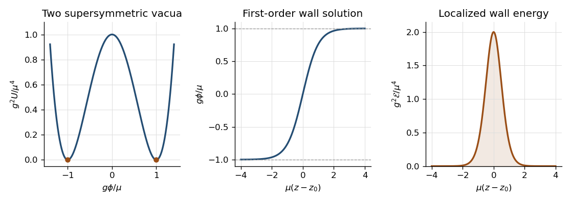
The wall breaks transverse translations: changing $z_0$ gives a normalizable scalar zero mode proportional to ${\varphi }^{\prime }(z)$. It also preserves only half the four real supercharges. In the chiral-fermion transformation, $F=-\overline{W^{\prime }}=-{\varphi }^{\prime }$ and the derivative term combine into a rank-half condition on the constant supersymmetry parameter, for example $ϵ=i{\sigma }^3\overline{ϵ}$ in a compatible Weyl convention. The orthogonal two real parameters are broken and generate localized fermion zero modes. One such profile satisfies $({\partial }_z+2g\varphi )f=0$, giving $f\propto {\mathrm{sech}}^2(\mu (z-z_0))$. The scalar and a three-dimensional Majorana fermion therefore form the low-energy wall multiplet. The domain-wall charge in N=1 supersymmetry is a boundary/tensor charge contributing to the extended algebra; the preserved combinations saturate $T=2|\Delta W|$. This avoids falsely applying the unextended particle-algebra argument of Question 3 to a wall with nonzero tension.

Promote the translation collective coordinate to a slowly varying worldvolume field $Y({\xi }^0,{\xi }^1,{\xi }^2)$. At wavelengths long compared with the wall thickness, its leading relativistic geometric action is the Dirac membrane actionIt is invariant under worldvolume reparametrizations and the target Poincaré group. In static gauge $X^i={\xi }^i$, $X^3=Y$, the matrix determinant lemma givesDirectly substituting the leading collective-coordinate profile into the scalar kinetic term gives the same coefficient, since $\int dz({\varphi }^{\prime }{)}^2=T/2$. Target Lorentz symmetry fixes the leading first-derivative nonlinear completion to the invariant area; finite-thickness physics can add higher-curvature terms. The area action is therefore a long-wavelength effective field theory, not an exact replacement for the microscopic wall at arbitrary momenta. Its embedding equation is ${\partial }_i(\sqrt{-h}{h}^{ij}{\partial }_j{X}^m)=0$.

For the four-dimensional supermembrane, extend the embedding to $(X^m(\xi ),{\theta }^{\alpha }(\xi ))$ with a four-real-component Majorana spinor. Pull back the invariant coframe of Question 7:Replacing $\partial X$ by $\Pi$ makes the area term invariant under rigid target supersymmetry, but does not yet give the appropriate fermionic gauge symmetry. Add a Wess-Zumino brane coupling to a superspace three-form potential $C_3$. In one orientation and matching normalization,The supermembrane closed four-form uses the distinct four-dimensional Fierz identity $(C{\gamma }_{mn}{)}_{(\alpha \beta }(C{\gamma }^n{)}_{\gamma \delta )}=0$. Differentiating $G_4$ reduces its coefficient to this symmetric tensor, so $d{G}_4=0$. A local potential therefore exists. Since the curvature is supertranslation invariant, the potential can vary by an exact form; its pullback integral is invariant modulo boundary terms. This is why the three-form $H_3$ of Question 7 is not itself the membrane field strength: integrating a membrane potential requires three-form degree and hence four-form curvature.

The required additional local fermionic gauge invariance is kappa symmetry. Define the worldvolume gamma matrices ${\gamma }_i={\Pi }_i^m{\gamma }_m$ andWith mostly-plus target signature, a local orthonormal worldvolume frame gives ${\Gamma }_{\kappa }={\gamma }_0{\gamma }_1{\gamma }_2$, so ${\Gamma }_{\kappa }^2=1$ and $\mathrm{tr}{\Gamma }_{\kappa }=0$. Thus $(1\pm {\Gamma }_{\kappa })/2$ are rank-two kappa symmetry projectors. The embedding variation gives $\delta {\Pi }_i^m=2i\delta \bar{\theta }{\gamma }^m{\partial }_i\theta$. The area variation is consequently proportional to $-2iT\sqrt{-h}\delta \bar{\theta }{\gamma }^i{\partial }_i\theta$. Contracting the displayed $G_4$ with the fermionic variation and using ${ϵ}^{ijk}{\gamma }_{ij}=2\sqrt{-h}{\Gamma }_{\kappa }{\gamma }^k$ gives the opposite Wess-Zumino contribution with an extra ${\Gamma }_{\kappa }$. Their sum is proportional toFor the boxed kappa variation, $\delta \bar{\theta }=\bar{\kappa }(1+{\Gamma }_{\kappa })$, so it vanishes by $(1+{\Gamma }_{\kappa })(1-{\Gamma }_{\kappa })=0$. Reversing membrane orientation reverses the Wess-Zumino sign and the matching projector. The cancellation fixes the relative charge magnitude to the tension; rigid supersymmetry alone would not fix it.

Worldvolume reparametrizations remove three of the four embedding scalars, leaving one transverse mode. Kappa symmetry removes half the four real embedding spinor components, leaving a two-component three-dimensional Majorana field, whose first-order equation has one on-shell fermionic polarization. The physical worldvolume modes are one scalar and one Majorana fermion, matching the wall zero modes. Without kappa symmetry the fermionic degrees would be doubled. A planar configuration preserves the target supersymmetries that can be compensated by the kappa projector, reproducing the wall's half-supersymmetry condition. This is the four-dimensional effective domain-wall interpretation of a supermembrane, rather than the eleven-dimensional M2-brane particle-content problem.

Use natural units and the Minkowski metric $g=\mathrm{diag}(1,-1,-1,-1)$. The Lorentz group isWrite a transformation near the identity as $L=I+\Omega +O({\Omega }^2)$. The defining relation gives ${\Omega }^{T}g+g\Omega =0$, so ${\omega }_{\mu \nu }=g_{\mu \rho }{\Omega }^{\rho }{}_{\nu }$ is antisymmetric. ChooseThere are $\left(\genfrac{}{}{0ex}{}{4}{2}\right)=\boxed{6}$ independent real parameters: three spatial rotations and three Lorentz boosts. Differentiating $(e^{t\Omega }{)}^{T}g{e}^{t\Omega }$ with respect to $t$ shows it is constant and equals $g$. Thus exponentiating these infinitesimal generators gives Lorentz transformations connected to the identity. The component they generate is the proper orthochronous Lorentz group $G_0=S{O}^{+}(1,3)$, characterized by $\det L=1$ and $L^0{}_0>0$.

The local exponential calculation alone establishes products of exponentials. The single-exponential assertion also holds here. Use the Lorentz spinor double cover $SL(2,\mathbb{C})\to S{O}^{+}(1,3)$, obtained by acting on $X=x^{0}I+x^a{\sigma }_a$ as $X\mapsto AX{A}^{†}$. Its determinant is the Minkowski norm. A lift $A$ with distinct eigenvalues $\lambda ,{\lambda }^{-1}$ is diagonalizable and has a traceless logarithm with eigenvalues $z,-z$, where $e^z=\lambda$. With repeated eigenvalues, choose between $A$ and $-A$ so that the lift is $I+N$ with $N^2=0$; its traceless logarithm is $N$. Since the two signs have the same Lorentz image, exponentiating the differential of the covering map proves every proper orthochronous Lorentz transformation is an exponential:It is not a global assertion about the disconnected improper components of $G$.

For Dirac spinors, choose gamma matrices satisfying the Clifford algebra $\{{\gamma }^{\mu },{\gamma }^{\nu }\}=2g^{\mu \nu }I$ and setThe Clifford relations giveThey also give the stipulated Lorentz commutator with every $M$ replaced by $\Sigma$: commute $\Sigma$ through the two gamma factors defining the other generator and collect the four terms. Consequently this is a representation of the Lie algebra of the Lorentz group, and exponentiation yieldsThe Dirac adjoint $\bar{\psi }={\psi }^{†}{\gamma }^0$ transforms as ${\bar{\psi }}^{\prime }=\bar{\psi }{S}^{-1}$, since $S^{†}{\gamma }^{0}S={\gamma }^0$.

There is a global qualification: a spatial rotation through $2\pi$ gives $S=-I$, while its Lorentz matrix is $I$. Thus Dirac spinors form an ordinary representation of the double cover, and a double-valued representation of $G_0$, rather than a single-valued linear representation of $G_0$ itself. Fermion bilinears are unaffected by this sign.

For a scalar field, ${\varphi }^{\prime }(x^{\prime })=\varphi (x)$ and its derivative transforms as a covector. A Lagrangian density must have all Lorentz indices contracted into scalars using invariant tensors; arbitrary scalar potentials are allowed. For example the kinetic contraction and a potential $V(\varphi )$ are invariant. Lorentz invariance by itself does not restrict the potential to quartic order: that restriction would be an additional four-dimensional power-counting requirement.

Define ${\gamma }^5=i{\gamma }^0{\gamma }^1{\gamma }^2{\gamma }^3$. It commutes with all ${\Sigma }^{\rho \sigma }$, so the axial current $j_5^{\mu }=\bar{\psi }{\gamma }^{\mu }{\gamma }^5\psi$ transforms as a vector under $G_0$. Hence all three proposed contractions are invariant under $G_0$. If invariance under parity or the full improper Lorentz group is also required, the distinction is:The axial current is a pseudovector: under an improper Lorentz transformation it has the extra determinant sign. The mixed derivative–axial contraction is therefore a pseudoscalar, while the square of the axial current has two cancelling signs. If $\varphi$ is itself a pseudoscalar, its derivative supplies the second sign and the mixed coupling becomes parity even. This is the axial derivative coupling and parity distinction; parity invariance must not be silently assumed from proper Lorentz invariance.

In four dimensions, $[\varphi ]=1$, $[\psi ]=3/2$ and $[{\partial }_{\mu }]=1$. The three operators have mass dimensions $4,5,6$, respectively. Thus the latter two require dimensionful couplings and are not power-counting renormalizable interactions, but this does not invalidate their Lorentz invariance or their use in an effective field theory.

The kinetic normalization fixes $[\Phi ]=(d-2)/2$, since a derivative has mass dimension one and the Lagrangian density has dimension $d$. Every differentiated field is still a field insertion. Hence the interaction has $n+r$ legs, not just $n$, and its vertex contains a homogeneous polynomial of degree $r$ in the attached momenta. Its coupling dimension isFor a connected Feynman diagram of this vertex type,The superficial momentum degree is now $D=dL-2I+rV$. Eliminating $I$ and $L$ givesso derivative-interaction scalar power counting yieldsThe same counting applies to tensor components with quantum field theory propagators scaling as $p^{-2}$; contractions, identities and cancellations can lower the actual degree. A coupling of negative mass dimension lets the superficial degree increase with the number of vertices, explaining the need for progressively higher-dimensional counterterms in a perturbative effective field theory.

Use $F_{\mu \nu }^a={\partial }_{\mu }{A}_{\nu }^a-{\partial }_{\nu }{A}_{\mu }^a+g{f}^{abc}{A}_{\mu }^b{A}_{\nu }^c$ and $\mathcal{L}=-F_{\mu \nu }^a{F}^{a\mu \nu }/4$. Its cubic and quartic Yang-Mills self-interactions areAntisymmetry of the Lie algebra structure constants lets the cubic expression also be written as $-g{f}^{abc}({\partial }_{\mu }{A}_{\nu }^a)A^{b\mu }{A}^{c\nu }$.

The cubic vertex has three fields and one derivative, corresponding to $n=2,r=1$ in part (b). The quartic vertex has four fields and no derivatives, corresponding to $n=4,r=0$. Their dimensions areWith both types present, the same Feynman diagram counting givesIn four dimensions both couplings are dimensionless, and the degree is bounded independently of vertex count. Gauge symmetry, implemented consistently after gauge fixing, restricts the ultraviolet counterterms to the allowed renormalizable gauge-invariant and gauge fixing/ghost structures. Thus the counting is consistent with perturbative renormalizability of ordinary four-dimensional Yang-Mills theory.

In six dimensions $[g]=-1$ and $[g^2]=-2$, giving $D=6-2E+V_3+2V_4$. Increasing the vertex count permits new divergent momentum structures and higher-dimensional operators without a finite closed list of renormalization parameters. Ordinary Yang-Mills theory is therefore power-counting renormalizable in four dimensions and nonrenormalizable in six dimensions. It can still be used in six dimensions as an effective field theory with a cutoff and higher-operator expansion; this conclusion concerns the usual perturbative theory.

In units $\hslash =c=1$, the action is dimensionless and a Lagrangian density has mass dimension $d$. The kinetic term therefore gives $2+2[\varphi ]=d$. Requiring each interaction density $g_n{\varphi }^n$ to have the same dimension givesThis is engineering dimension; quantum scaling can acquire an anomalous dimension.

For a connected Feynman diagram with no derivative interactions, each independent loop integration contributes $d$ powers of momentum, and each internal scalar propagator contributes $-2$. Thus its superficial degree of divergence is $D=dL-2I$. Let $V={\sum }_n{V}_n$. A connected graph has $L=I-V+1$ independent cycles, and counting the half-edges incident on vertices gives $2I+E={\sum }_{n}n{V}_n$. Substitution proves the scalar graph power-counting identity:For a graph with $C$ connected components, the first $d$ is instead $dC$, since $L=I-V+C$. The printed expression therefore uses the usual connected-graph convention. This is the overall degree under simultaneous rescaling of all loop momenta. Subgraphs can still have ultraviolet divergences when the whole graph has $D<0$, so their counterterms must be subtracted before declaring an integral finite.

When all retained couplings have nonnegative dimension, only finitely many external-leg/derivative structures can have nonnegative degree. Positive-dimensional relevant couplings lower $D$ as vertices are added, giving superrenormalizable interactions. Zero-dimensional marginal couplings give power-counting renormalizable interactions. Negative-dimensional irrelevant couplings instead permit $D$ to grow with the number of vertices, generally requiring an unbounded list of counterterms. Such nonrenormalizable interactions can still define an effective field theory to any fixed order in a low-energy expansion.

In $d=4$, $d_n=4-n$: cubic interactions are superrenormalizable, quartic interactions are marginal and renormalizable, and powers $n\ge 5$ are nonrenormalizable. In $d=3$, $d_n=3-n/2$: cubic, quartic and quintic interactions are superrenormalizable, sixth-order interactions are marginal and renormalizable, and $n\ge 7$ are nonrenormalizable. This is a power-counting classification, not a guarantee that an odd highest-power potential is bounded below. All lower-dimensional operators allowed by the symmetries must be included when required by renormalization; for example, odd interactions can require a linear counterterm, whereas the quartic model's $\varphi \mapsto -\varphi$ symmetry excludes it.

Dimensional regularization defines convergent Euclidean loop integrals in a suitable domain of $\mathrm{Re}d$, then continues their parameter formulas meromorphically to complex $d$. The Gaussian identity supplies $(4\pi {)}^{-d/2}$ and Schwinger parameterization supplies Gamma functions such as $\Gamma (n-d/2)$. Their poles encode the ultraviolet singularities near physical dimension. Noninteger complex $d$ is an analytic regulator of amplitudes, not a literal space with a noninteger number of coordinates. Masses or nonexceptional external momenta distinguish ultraviolet poles from infrared poles; scaleless integrals vanish in this convention and can hide that distinction.

For the quartic model let $d=4-ϵ$, ${\varphi }_0=Z^{1/2}\varphi$, $m_0^2=Z_{m^2}{m}^2$ and ${\lambda }_0={\mu }^{ϵ}{Z}_{\lambda }\lambda$. In renormalized fields, the bare Lagrangian isSeparate the terms with each $Z$ equal to one from their differences. The differences are field, mass and quartic counterterms. After subtracting divergent subgraphs, the remaining ultraviolet pole of a proper graph is a local polynomial in its external momenta. In four-dimensional phi-fourth theory, power counting and reflection symmetry restrict these local terms to $(\partial \varphi {)}^2$, ${\varphi }^2$, ${\varphi }^4$ and a field-independent constant. Choosing the Laurent coefficients of the three renormalization factors recursively cancels these poles at every perturbative order. The constant vacuum term is removed by the zero-source normalization. This is an order-by-order finite renormalized expansion, not a claim of convergence of the perturbation series.

The source renormalization of a scalar generating functional follows directly from rewriting the source coupling in bare variables:A general source attached to a single elementary field needs this field renormalization; its connected correlations are the ordinary renormalized Green functions. Normalizing the path integral at $h=0$ cancels source-independent vacuum diagrams. Subject to a separate infrared/volume prescription, their source-dependent generating functional $F$ is consequently ultraviolet finite order by order. For a constant source, this statement is interpreted as a formal connected expansion or a vacuum density, not as an automatically finite total logarithm in infinite spacetime.

Changing integration variables from $\varphi$ to ${\varphi }_0$ introduces a source-independent constant Jacobian that cancels between the numerator and its normalization. The resulting normalized integral depends only on ${\lambda }_0,m_0^2,h_0$ and fixed physical boundary/volume data. ThusDefine all scale derivatives at these fixed bare quantities:In a mass-independent subtraction scheme, logarithmic differentiation of the bare relations givesThe factors contain regulator poles, but the combinations determining the physical renormalization group functions have finite limits. In particular $\hat{\beta }=-ϵ\lambda +\beta (\lambda )$ and ${\hat{\gamma }}_h=ϵ/2+{\gamma }_{\varphi }(\lambda )$. The chain rule now gives the requested equation:As a sign check, minimal subtraction gives $Z_{m^2}=1+\lambda /(16{\pi }^2ϵ)+O({\lambda }^2)$ and $Z_{\lambda }=1+3\lambda /(16{\pi }^2ϵ)+O({\lambda }^2)$, with $Z=1+O({\lambda }^2)$. Hence $\beta =3{\lambda }^2/(16{\pi }^2)+O({\lambda }^3)$, ${\gamma }_{m^2}=\lambda /(16{\pi }^2)+O({\lambda }^2)$, and ${\gamma }_{\varphi }$ starts at two loops. The positive signs agree with the tadpole subtraction and the three four-point channels.

The dimensional rewriting needs care. The chosen source normalization gives $[h]=3$, $[m^2]=2$, and $[\lambda ]=0$, so $m^2/{\mu }^2$ and $h/{\mu }^3$ are the natural dimensionless parameters. For the full source functional, spacetime arguments must also be rescaled: with $y=\mu x$, write $\varphi (x)={\mu }^{(d-2)/2}\psi (y)$ and $\tilde{h}(y)={\mu }^{-3}h(y/\mu )$. The dimensionless functional then depends on $\lambda ,m^2/{\mu }^2$, the rescaled source profile, and the rescaled integration domain.

For a literal uniform source in a fixed physical spacetime volume ${\mathcal{V}}_d$, the uniform-source vacuum functional and spacetime volume relation is insteadFor example, even at $\lambda =0$ and $m^2>0$, completing the square for the constant mode givesThus the printed three-argument rewriting of the total $F$ suppresses necessary volume/source-profile data. It is valid as a dimensional shorthand only with those data understood; a dimensionless density has the three arguments, while its scale equation includes its engineering dimension. At infinite volume, the total constant-source logarithm is generally extensive and infinite even after ultraviolet renormalization.

The massless renormalization-group characteristics with a source solve the requested flow directly, independently of this notational issue. Since the mass flow is proportional to $m^2$, its zero value remains zero. Starting at a reference scale ${\mu }_{\ast }$, solveThenwith any physical volume or source-shape data retained. Where $\hat{\beta }\ne 0$, the running quantities are determined byThese equations transport matching data at one scale to any other scale on the same flow trajectory. At a zero of the beta function use the differential equations themselves, rather than divide by zero.

For the uniform-source density, set $y=h/{\mu }^3$ and $m^2=0$. At $d=4$ the corrected dimensionless equation and its local characteristic solution areThe arbitrary function $\Psi$ is fixed by boundary/matching data. If the volume is retained as a dimensionless argument $v={\mu }^4{\mathcal{V}}_4$, the full dimensionless functional obeys the same transport operator with $4v{\partial }_v$ in place of the additive $4$ term; extensivity makes the two statements equivalent. Massless zero-momentum source expansions can also have infrared singularities, so this RG solution is formal until an infrared prescription or a suitable background expansion is chosen.

An ultraviolet fixed point is a zero of the beta functions approached by the dimensionless couplings as $\mu \to \infty$. Near a single-coupling fixed point ${\lambda }_{\ast }$, perturbations obey $\delta \lambda \propto {\mu }^{{\beta }^{\prime }({\lambda }_{\ast })}$, so ${\beta }^{\prime }<0$ gives attraction in that direction. In four-dimensional quartic scalar theory, the positive one-loop beta function makes positive small coupling grow toward the ultraviolet: $1/\lambda (\mu )=1/\lambda ({\mu }_{\ast })-[3/(16{\pi }^2)]\log (\mu /{\mu }_{\ast })$. This exhibits a perturbative Landau pole, not an interacting ultraviolet fixed point. A perturbative result does not exclude hypothetical strong-coupling behavior beyond its regime.

Use natural units and the Minkowski metric $g_{\mu \nu }=\mathrm{diag}(1,-1,-1,-1)$. A massive spin-one particle has three physical particle polarizations, whereas a massless gauge boson has two. Giving a vector a mass must account for this extra longitudinal state while preserving a positive physical state space, controlled high-energy scattering and, if a fundamental perturbative theory is sought, renormalizability.

At the free-field level there is no inconsistency. The Proca actiongives the Proca equation ${\partial }_{\nu }{F}^{\nu \mu }+m^2{A}^{\mu }=0$. Taking its divergence gives $m^2{\partial }_{\mu }{A}^{\mu }=0$, and then $(\square +m^2)A^{\mu }=0$. For $m>0$ the divergence constraint removes one of the four components, leaving three positive-norm physical modes. The time component is constrained, rather than an independent negative-norm propagating oscillator. The mass term does, however, change under $A_{\mu }\mapsto A_{\mu }+{\partial }_{\mu }\omega$, so the ordinary massless gauge invariance is no longer manifest.

The difficulty becomes acute for generic interactions. Inverting the quadratic operator gives the Proca propagatorThe longitudinal part approaches order $1/m^2$ at large momentum, rather than falling as $1/k^2$. Thus the usual ultraviolet power counting deteriorates. There is a parallel external-state problem: for $p^{\mu }=(E,\mathbf{p})$,Longitudinal external legs can generate powers of $E/m$ in a scattering amplitude. These are the high-energy obstruction for a hard vector mass. Conserved Abelian currents can remove dangerous contractions, so one should not conclude that every massive-vector interaction is impossible.

For a massive non-Abelian vector with gauge-like cubic and quartic couplings, cancellations among diagrams remove the largest powers, but without a suitable additional sector longitudinal scattering still grows like $s/v^2$, where $v$ is the symmetry-breaking scale. A partial-wave coefficient is then of order $s/(16\pi v^2)$. Partial-wave unitarity requires its real part to remain bounded, so perturbation theory fails at energies of order the electroweak scale times a modest loop factor, around the TeV scale for electroweak vectors. This is a limit on the perturbative description, not a proof that a low-energy massive-vector effective field theory is inconsistent.

The Higgs mechanism supplies a weakly coupled completion. For an Abelian example, take a complex scalar field withLocally write $\varphi =(v+h)e^{i\chi /v}/\sqrt{2}$. Its gauge-covariant kinetic term becomesThe combination is invariant under $A_{\mu }\mapsto A_{\mu }+{\partial }_{\mu }\omega$, $\chi \mapsto \chi +gv\omega$. In unitary gauge $\chi =0$, it contains $m^2{A}_{\mu }{A}^{\mu }/2$ with $m=gv$, as well as the correlated $hAA$ and $hhAA$ interactions. The two original gauge polarizations and two real scalar components become three massive-vector polarizations and one radial Higgs boson. The would-be Goldstone boson supplies the longitudinal state. This counting explains why the Goldstone theorem for spontaneously broken global symmetries does not imply an extra physical massless particle here. Local gauge symmetry is a redundancy; choosing a Higgs background after gauge fixing does not explicitly break the gauge invariance of the action.

The extra scalar interactions also repair high-energy scattering. By the Goldstone-boson equivalence theorem, the leading longitudinal-vector amplitude can be computed using the would-be Goldstone bosons. For a charged-to-neutral channel in the linear scalar model, the scalar contact and radial-exchange terms giveThis Higgs cancellation in longitudinal vector scattering removes the uncontrolled $s/v^2$ growth. It also shows why a very large scalar self-coupling would itself make perturbation theory unreliable; introducing a scalar is not a license to ignore partial-wave unitarity.

Although the unitary gauge propagator looks like the badly behaved Proca propagator, renormalizability is conveniently established in an R-xi gauge. Using Cartesian scalar fluctuations, the quadratic mixing is $-m{A}_{\mu }{\partial }^{\mu }\chi$. The gauge-fixing term $-(\partial \cdot A+\xi m\chi {)}^2/(2\xi )$ cancels it and givesAt fixed finite $\xi$ this falls as $1/k^2$. The would-be scalar modes and Faddeev-Popov ghosts remain in intermediate calculations. Gauge identities, organized through BRST symmetry, make unphysical states cancel from physical amplitudes and constrain counterterms to the gauge-invariant renormalizable form. With a renormalizable scalar sector and cancellation of gauge anomalies, spontaneously broken gauge theory is renormalizable and unitary on its physical states; the bosonic construction is demonstrated in the original massive Yang-Mills renormalizability proof. The ultraviolet limit and $\xi \to \infty$ limit do not commute, so the unitary-gauge numerator alone is not a valid disproof of this result.

In the Standard Model, a Higgs doublet breaks the manifest electroweak group from $SU(2{)}_L\times U(1{)}_Y$ to $U(1{)}_{\mathrm{em}}$. The scalar kinetic term yieldsThree scalar directions supply the longitudinal polarizations of $W^{\pm }$ and $Z$, while the unbroken electromagnetic generator leaves the photon massless. The radial Higgs boson remains physical.

There is an important Abelian alternative. The Stueckelberg mechanism introduces a scalar with ${\mathcal{L}}_{\mathrm{mass}}=(m{A}_{\mu }-{\partial }_{\mu }\chi {)}^2/2$, invariant under $A\mapsto A+\partial \omega$, $\chi \mapsto \chi +m\omega$. With suitable conserved-current couplings this can describe a renormalizable massive Abelian gauge theory without a radial Higgs particle. A naive non-Abelian analogue involves a nonlinear group-valued scalar and derivative interactions suppressed by inverse powers of the symmetry-breaking scale; it is generally an effective field theory, not a power-counting-renormalizable substitute. Strongly coupled or composite sectors can provide other completions. A free vector mass is consistent; the central problem is obtaining the longitudinal state and its interactions in a theory with controlled ultraviolet behavior and physical unitarity.

Kaluza-Klein theory explains apparently four-dimensional physics as the low-energy limit of a higher-dimensional theory with compact spatial directions. In units $\hslash =c=1$, take a circle coordinate $y\sim y+2\pi R$. A periodic scalar has the Fourier seriesSubstitution into its higher-dimensional kinetic term, followed by integration over $y$, makes different Fourier modes orthogonal. The internal derivative contributes $n^2/R^2$ to the lower-dimensional squared mass, soThe quantized internal momentum produces the Kaluza-Klein tower. A real higher-dimensional field satisfies ${\varphi }_{-n}={\varphi }_n^{\ast }$; the tower does not introduce independent complex modes for both signs. More general compact spaces replace $n^2/R^2$ by Laplacian eigenvalues, with boundary conditions determining the spectrum.

At energies $E\ll R^{-1}$, nonzero Kaluza-Klein modes cannot be produced and may be integrated out, leaving a four-dimensional effective field theory. Dimensional reduction retains the zero modes at leading order; integrating out the massive modes also generates interactions suppressed by the Kaluza-Klein compactification scale. The higher-dimensional metric decomposes into a four-dimensional metric, vectors from mixed components, and scalar fields from internal components. For a circle, these include an Abelian gauge field and a radion. Internal coordinate shifts induce the vector's gauge symmetry, while the radion describes the radius. Pure circle reduction alone does not automatically give the chiral matter spectrum of the Standard Model.

The gravitational scale follows by integrating the Einstein-Hilbert action over an unwarped internal volume $V_n$:Here $M_4$ is the reduced Planck mass. For $n$ equal circle radii, $V_n=(2\pi R{)}^n$. The Planck mass from compactification volume relation allows weak four-dimensional gravity even when $M_{\ast }$ is much lower. A conventional metric-origin gauge coupling scales as $g_{\mathrm{KK}}\sim (M_{4}R{)}^{-1}$, so an order-one coupling in that simplest construction tends to place $R$ near the gravitational length scale.

In the brane-world scenario, ordinary matter and its gauge fields can instead be localized on a three-dimensional spatial brane, while gravity explores the bulk. The absence of ordinary-matter excitations along the extra dimensions then permits larger radii than a model in which all fields propagate there. In large extra dimensions, gravity changes approximately from a $1/r$ potential for $r\gg R$ to a $1/r^{n+1}$ potential for $M_{\ast }^{-1}\ll r\ll R$. For illustration, $M_{\ast }$ of order a TeV and $n=2$ give $R$ of order $0.1$ mm; one extra dimension would require an astronomically large radius.

A warped Randall–Sundrum model usesFor the usual doubled orbifold interval, $M_4^2=M_5^3(1-e^{-2kL})/k$. The relevant lengths are the bulk curvature radius $k^{-1}$, the proper separation $L$, and the inverse warped excitation scale, of order $(k{e}^{-kL}{)}^{-1}$. Thus the first mass need not equal $1/L$. Compact volume dilutes gravity; warping redshifts local masses. Both mechanisms require consistent field localization and radius stabilization; choosing a large radius or separation is not itself a dynamical explanation of it.

A renormalizable quantum field theory requires only finitely many independent field and parameter redefinitions to remove regulator dependence from its perturbative correlation functions, order by order. The allowed local counterterms must close within that finite set; it is not necessary that the unrenormalized integrals be finite.

In four spacetime dimensions the kinetic term fixes the mass dimension of $\varphi$ to one. A coefficient multiplying ${\varphi }^k$ therefore has dimension $4-k$. Power counting excludes couplings of negative mass dimension for perturbative renormalizability. For a single scalar with a conventional nonderivative polynomial potential, the allowed form isThe constant controls vacuum energy and the linear term a possible tadpole. A field-reflection symmetry can remove the odd terms but is not necessary for renormalizability. Terms of degree above four generally require an infinite tower of counterterms when treated as fundamental interactions; they can instead be used in an effective field theory. Stability of the potential is a separate requirement, for example a positive quartic leading term, and should not be confused with the power-counting criterion.

For a graph with $E$ external scalar lines, $I$ internal lines, $L$ loops and $V_k$ vertices of degree $k$, the superficial ultraviolet divergence degree is $\omega =4L-2I$. The identities $L=I-{\sum }_k{V}_k+1$ and $2I+E={\sum }_{k}k{V}_k$ giveWhen every $k\le 4$, only the finitely many low-point local divergences, including the kinetic term, can require subtraction. Subdivergences are removed recursively by the same local counterterms. A vertex with $k>4$ instead permits arbitrarily high divergence degrees as more such vertices are added. This explains the restriction rather than merely asserting it.

The bare Lagrangian density is written in terms of regulator-dependent bare quantities, before taking the regulator away:The coefficients in $V_B$ are related to the renormalized parameters by regulator-dependent redefinitions. The wave-function renormalization supplies a kinetic counterterm. In dimensional regularization $d=4-ϵ$, a quartic coupling has a bare relation of the form ${\lambda }_B={\mu }^{ϵ}[\lambda +\delta \lambda (\lambda ,ϵ)]$, with field factors incorporated according to the chosen definition. The bare parameters and bare correlation functions are held fixed when changing the renormalization scale.

Even without a physical mass, interacting loop subtractions require a reference scale $\mu$ to define the renormalized dimensionless coupling and field normalization. Finite logarithms then involve dimensionless combinations such as $\mu |x_r-x_s|$ or $p^2/{\mu }^2$. This scale is a subtraction convention, not a new physical mass parameter. Its explicit dependence is compensated by the running coupling and field normalization.

Let $G_n=⟨\varphi (x_1)\cdots \varphi (x_n)⟩$ at separated points. Its bare counterpart satisfies $G_{B,n}=Z_{\varphi }^{n/2}{G}_n$. DefineDifferentiating $G_{B,n}$ at fixed bare theory givesThis Callan-Symanzik equation expresses independence of the arbitrary subtraction scale. The renormalization-group beta function describes the compensating coupling change; the field-renormalization anomalous dimension describes the compensating rescaling of each insertion. Coincident composite insertions would require their own additional renormalization, rather than automatically obeying this separated-point equation.

For the two-point function, set $z=p^2/{\mu }^2$ and $t=\frac{1}{2}\log z$. We consider large positive spacelike $p^2$, with continuation to other momenta as required. The dimensionless propagator factor obeysDefine $\bar{g}(0)=g$ and $d\bar{g}/dt=\beta (\bar{g})$. The renormalization-group characteristic solution for a two-point function isTo verify it, the running-coupling flow has $\beta (g){\partial }_g\bar{g}(t)=\beta (\bar{g}(t))$. Also, $\beta (g){\partial }_g{\int }_0^t\gamma (\bar{g}(s))ds=\gamma (\bar{g}(t))-\gamma (g)$. Applying ${\partial }_t-\beta (g){\partial }_g$ to the displayed expression therefore gives $2\gamma (g)d$, exactly the required differential equation. The boundary value $d(1,g)$ records the renormalization condition. This shows how the ultraviolet behaviour is determined by the coupling trajectory and its accumulated anomalous dimension: it can approach zero coupling, a nonzero fixed point, or a finite-scale singularity, depending on $\beta$.