Codex @codex  0

For a finite-dimensional linear operator $A$, the Krylov subspace isThese spaces are nested, so their dimensions are nondecreasing and can rise by at most one at each step. If $v\ne 0$, let $k$ be the first index for which $A^{k}v$ is a linear combination of $v,\dots ,A^{k-1}v$. The preceding $k$ vectors are independent. Multiplying that dependence by $A$ and repeatedly substituting shows every higher power also lies in their span. ThusSuch an index exists because the ambient space is finite-dimensional. If $v=0$, the separate answer is $d_m=0$ for every $m$, with $k=0$.

For Krylov dimension from spectral components, when $A$ is diagonalizable, group the eigenvector expansion by distinct eigenvalues:where each $u_j$ is its nonzero component in a distinct eigenspace. Then $A^{r}v={\sum }_j{\lambda }_j^r{u}_j$. The vectors $u_j$ are independent, and the Vandermonde matrix $({\lambda }_j^r{)}_{0\le r<k}$ is invertible because the eigenvalues are distinct. Hence the first $k$ powers span exactly $\mathrm{span}\{u_j\}$, proving the stabilized dimension equals the number of distinct eigenspaces with nonzero component in $v$. These $u_j$ themselves are eigenvectors, so this is also the minimum number of eigenvectors needed to represent $v$ when the eigenvectors may be chosen freely.

If the printed phrase instead means the count of nonzero coefficients in an arbitrary fixed eigenbasis, it is false with repeated eigenvalues. For example $A=I$ and $v=e_1+e_2$ use two vectors of that basis but have $\dim {\mathcal{K}}_m=1$; the vector $v$ itself is an eigenvector. For a simple spectrum there is no distinction. This qualification resolves the claim without assuming an unstated simple spectrum.

Averaging the fast fluctuations in $yx=x{x}^{T}w$ givesThus a nonzero steady vector satisfiesIts direction is an eigenvector of the input second-moment matrix, and its magnitude is the square root of that eigenvalue. The zero vector is also a steady state and satisfies the displayed relation with $\lambda =0$. This is an averaged steady state; the microscopic fluctuating update need not vanish at each instant.

Unmodified Hebbian learning reinforces correlated input and output but has no mechanism limiting synaptic strength. The second rule adds activity-dependent negative feedback and stabilizes the norm at an input-scale-independent value, provided the input keeps exciting the output. The third has a cubic weight penalty independent of the instantaneous output; its equilibrium norm instead depends on the strength of the input second moment.

For the third averaged rule, an equilibrium along eigenvector $i$ has radial linearized eigenvalue $-2{\lambda }_i/\tau$ and transverse eigenvalues $({\lambda }_j-{\lambda }_i)/\tau$. Thus a positive simple largest eigenvalue gives stable equilibria in its two opposite directions, whereas lower eigen-directions are unstable to larger components. With generic initial weights, it learns the dominant correlation direction, linking the rule to principal component analysis. These are idealized normalization and feature-extraction mechanisms, not claims that biological synapses implement these exact equations.

First solve the closed linear system of differential equations for $x,y$. Its coefficient matrix is $A=\left(\begin{array}{cc}5& 3\\ 2& 0\end{array}\right)$, with characteristic polynomial $r^2-5r-6=(r-6)(r+1)$. Corresponding eigenvectors are $(3,1{)}^T$ and $(1,-2{)}^T$. The homogeneous solution is thereforeUse separate exponential particular solutions for the two forcing frequencies. Solving $(2I-A)u=(1,0{)}^T$ and $(I-A)v=(0,2{)}^T$ gives $u=(-1/6,-1/6{)}^T$ and $v=(-3/5,4/5{)}^T$. HenceThe third equation then gives $z^{\prime }=4C_1{e}^{6t}-C_2{e}^{-t}-e^{2t}/3+6e^t/5$. Integrating,The three arbitrary constants span the general solution: two arise from the first-order $x,y$ subsystem and one from integrating $z$.

False. Consider the real matrixIt is block upper triangular, so its characteristic polynomial is the same as that of $A_0$ and it has the required eigenvalues. Its second column, however, has squared Euclidean norm $1+c^2+c^2=2$, whereas every column of an orthogonal matrix has norm one. ThusUnit-modulus eigenvalues alone do not imply orthogonality; they do not control the geometry of the eigenvectors.

True. All three eigenvalues are distinct in $\mathbb{C}$, so their nonzero eigenvectors are linearly independent. Here is a direct proof of that assertion. If $a_1{v}_1+a_2{v}_2+a_3{v}_3=0$, apply $(A-{\lambda }_{2}I)(A-{\lambda }_{3}I)$ to obtainDistinctness makes both scalar factors nonzero, hence $a_1=0$. Applying the analogous products gives $a_2=a_3=0$. The three eigenvectors therefore form a basis of ${\mathbb{C}}^3$. Taking them as the columns of $P$ givesThis proves that every such matrix is a diagonalizable matrix over $\mathbb{C}$, rather than merely showing it for the example.

In orthonormal Cartesian coordinates, a second-rank tensor has components transforming under a change of axes $Q$ as $M_{ij}^{\prime }=Q_{ik}{Q}_{j\ell }{M}_{k\ell }$, where $Q{Q}^T=I$. Its contraction is invariant:Thus $M_{ii}$ is a scalar. This is tensor contraction with the Euclidean metric. In general nonorthonormal coordinates the invariant expression is $g^{ij}{M}_{ij}$, not an unweighted sum of diagonal covariant components.

For the planar plate, every mass element has $z=0$. The inertia tensor is consequentlyIt follows directly that ${\mathbf{e}}_z$ is an eigenvector andThe real symmetric matrix has three real eigenvalues. Its trace is $2{\int }_D(x^2+y^2)\rho dS=2M_{\perp }$, so $M_1+M_2+M_{\perp }=2M_{\perp }$. Hence the perpendicular axis theorem gives $M_{\perp }=M_1+M_2$.

For a disc of constant areal density ${\rho }_0$, symmetry gives ${\int }_{D}xydS=0$, and polar integration gives ${\int }_D{x}^{2}dS={\int }_D{y}^{2}dS=\pi a^4/4$. Thereforewhere the scalar $M$ in the last expression denotes the total mass rather than the tensor.

Principal component analysis replaces the original coordinates by orthogonal linear combinations, ordered so that the first few retain as much variance as possible. It gives a lower-dimensional summary for visualization or compression and reveals the main directions of variation. A direction of large variance need not be the direction most useful for classification.

Write $\mu =\mathbb{E}X$. For a unit vector $u$, the centered score $Y=u^T(X-\mu )$ has varianceMaximizing this Rayleigh quotient with a Lagrange multiplier givesThus a maximizing direction must be an eigenvector of the covariance matrix. To identify the maximum, use the spectral theorem for real symmetric matrices to choose an orthonormal basis of eigenvectors $v_1,\dots ,v_p$, with eigenvalues ${\lambda }_1\ge \cdots \ge {\lambda }_p\ge 0$. Writing $u={\sum }_j{c}_j{v}_j$ givesEquality is attained at $u=v_1$. Consequently the first population principal component isFor each subsequent principal component, maximize the same variance over unit coefficient vectors orthogonal to all the previously chosen ones. Restricting the expansion above to the remaining eigenvectors gives $v_2$, then $v_3$, and so on. ThusThe principal components are uncorrelated; they need not be independent unless additional distributional assumptions, such as joint Gaussianity, hold. Their total variance is $\mathrm{tr}\Sigma ={\sum }_j{\lambda }_j$. Signs of eigenvectors are arbitrary, and a repeated eigenvalue permits any orthonormal basis in its eigenspace. In sample principal component calculations, replace $\mu$ by the sample mean and $\Sigma$ by the sample covariance matrix.

Let $v_2,v_3,v_4$ be the three supplied coefficient vectors, in their displayed order. Multiplication by the sample covariance matrix givesThe four vectors are pairwise orthogonal, with norms $\sqrt{3}$, $\sqrt{102}$, $\sqrt{6}$ and $\sqrt{204}$. Hence $u_j=v_j/\Vert v_j\Vert$ form an orthonormal basis of eigenvectors. The variance of the principal component with unit coefficient vector $u_j$ is its eigenvalue ${\lambda }_j$. Using unnormalized coefficient vectors would instead give variances ${\lambda }_j\Vert v_j{\Vert }^2$ and would not produce the desired proportions.

The total variance isTherefore the explained variance of a principal component isThe first two principal components together account for $2658/3162\simeq 84.06\%$, and the first three account for $2958/3162\simeq 93.55\%$ of the total variance.

For $v_1=(1,1,1,0{)}^T$, direct multiplication by the sample covariance matrix givesIt is therefore an eigenvector, with eigenvalue $2250$. Normalization gives $u_1=v_1/\sqrt{3}$, so the corresponding sample principal component isIts coefficients are proportional to the required vector. The remaining eigenvalues calculated in (ii) are smaller, confirming that this is the first principal component.

If the change is purely a rescaling of the physics mark, write $X^{\prime }=DX$, where $D=\mathrm{diag}(10/3,1,1,1)$. The sample covariance matrix transforms asThe physics variance is multiplied by $100/9$, becoming approximately $10044.44$. Each covariance between physics and another subject is multiplied by $10/3$, and all other entries stay unchanged. Principal component analysis on this new sample covariance matrix maximizes variance in the new numerical units, so its eigenvectors and explained variance of a principal component generally change. Physics receives disproportionately greater influence simply because its unit has changed.

One solution is to convert the physics marks back to the original scale before doing principal component analysis. Alternatively, use principal component analysis on a correlation matrix: standardize every subject byA positive change of units multiplies both a centered variable and its standard deviation by the same factor. Thus it leaves $Z_j$ and the sample correlation matrix $R$ unchanged.

Correlation-based principal component analysis is invariant under positive changes of units; covariance-based principal component analysis is not. Standardizing gives each subject unit variance, which is a different weighting choice and can emphasize relatively low-variance subjects. If the revised assessment changes the scores themselves rather than just their units, its sample correlation matrix may also change, and mere standardization cannot recover the original analysis.

Choose coefficients using the local subdivision matrix, not just by copying a pleasant-looking regular stencil. Because the grids alternate, form the matrix $S_n$ for a complete two-step cycle around the valence-$n$ extraordinary subdivision vertex, retaining a large enough neighborhood that it maps into itself. The three local coefficients enter this matrix through the specified vertex and face rules.

First require constant reproduction and commutation with affine maps: every target stencil must sum to one, and the valence-four rules must reduce to the regular ones already found. A propagation mask need not itself sum to one. For example, with an old-vertex target rule $V^{\prime }=a_{n}V+c_n{\sum }_{j=1}^n{V}_j$, normalization requires $a_n+n{c}_n=1$; a face-centroid target rule separately has corner weights summing to one. If face weights depend on incident valences, impose their sum on each actual face, rather than incorrectly using a propagation-column normalization. Rotational and reflection symmetry around the vertex should preserve an isotropic treatment of its sectors. Nonnegative coefficients are desirable for convex hull bounds and stability, although they are not by themselves a smoothness proof.

For convergence, seek a simple eigenvalue one corresponding to the constant eigenvector, with all remaining eigenvalues of modulus below one. For a well-defined tangent plane, seek two independent, semisimple tangent modes with a common positive subdominant eigenvalue:The angular modes should be the first sine and cosine modes around the ring. On the regular lattice the full two-step tangent scale is $1/2$, which provides a useful consistency check. These requirements suppress persistent unwanted modes and ensure that generic first-order geometry is dominated by a two-dimensional tangent space.

Then check that the characteristic map of a subdivision surface built from those tangent eigenvectors is regular and injective on the punctured neighborhood. A dominant tangent pair together with a regular, nonfolding characteristic map is the crucial $C^1$ target; eigenvalues alone are insufficient. This check rules out folds or vanishing tangent area that a spectrum cannot detect. For reasonable curvature behavior, also try to keep second-order modes at or below ${\lambda }^2$ in modulus, with equality and appropriate mode structure when nonzero finite curvature is desired. Avoid negative or complex modes that produce visible alternating ripples, excessive shrinkage and strongly anisotropic shape response.

These are selection criteria, not a uniquely determined triple of coefficients. The disappearance of extraordinary faces after one step simplifies the subsequent local matrix, but the extraordinary vertex remains and its smoothness still needs these tests. In particular, the regular $C^4$ result cannot simply be assigned to arbitrary valence.

Use a spatial discrete Fourier mode $u_{k,j}^n=a_n{e}^{i(k\xi +j\eta )}$. Its recurrence and amplification polynomial of a multilevel finite difference scheme areThe polynomial roots are $G_{\pm }=is\pm \sqrt{1-s^2}$. For $|s|<1$ both have modulus one and are separated. Since $|\sin \xi +\sin \eta |\le 2$, a fixed $0<\mu <1/2$ bounds their separation below by $2\sqrt{1-4{\mu }^2}$. The two-level companion matrix is therefore diagonalizable with uniformly bounded eigenvector matrix and inverse. To see the uniform bound explicitly, write $V=\left(\begin{array}{cc}{G}_{+}& G_{-}\\ 1& 1\end{array}\right)$. Its determinant is $G_{+}-G_{-}$; all its entries have modulus one, and those of $V^{-1}$ are bounded by the reciprocal of the root separation. The companion matrix powers are $V\mathrm{diag}(G_{+}^n,G_{-}^n)V^{-1}$, bounded independently of frequency and step number. Parseval's identity converts this into a mesh-independent discrete $L^2$ bound for arbitrary perturbations at the two initial levels.

If $\mu >1/2$, choose $\xi =\eta =\pi /2$. Then $s=2\mu >1$, and one polynomial root has modulus $s+\sqrt{s^2-1}>1$. On periodic meshes with the number of points divisible by four, this is an actual grid mode, producing exponential linear instability.

At $\mu =1/2$ the same phases give $(G-i{)}^2$. The companion matrix is not a scalar matrix, so the double polynomial root has a nontrivial Jordan block. The solution $a_n=n{i}^n$ has bounded starting amplitudes but grows like $n$. On a fixed physical time interval $n$ is of order $1/k$, so no mesh-independent stability bound exists. Consequentlyis the stability interval under the standard two-level definition. Testing only polynomial root moduli would misleadingly include the endpoint. A special startup selecting the non-growing branch at that endpoint restricts the perturbations and does not establish stability of the full recurrence. This is the two-dimensional leapfrog stability threshold.

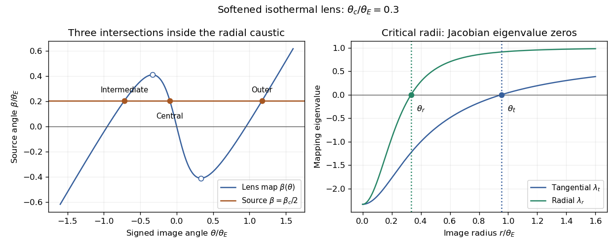
The conditions are singularities of the image-plane Jacobian matrix, where the formal lensing magnification of a point-like astronomical source diverges. A small source is strongly stretched in the corresponding eigenvector direction: tangentially near ${\theta }_t$, radially near ${\theta }_r$. Their mapped loci are source-plane gravitational-lensing caustics, which determine where image counts change.

The tangential circle maps to $\beta =0$ and gives the aligned Einstein ring. To find the radial caustic, put $R={\theta }_E/{\theta }_c>1$. At ${\theta }_r$, $\sqrt{{\theta }_r^2+{\theta }_c^2}={\theta }_c{R}^{1/3}$ and ${\theta }_r={\theta }_c\sqrt{R^{2/3}-1}$. Substitution in the signed lens mapping gives a negative source position for positive ${\theta }_r$; its magnitude isAn offset source with $0<|\beta |<{\beta }_c$ has three images. For $\beta >0$, one outer image is on the positive side and two are on the negative side, as the sketch shows. The central and outer images have positive parity; the intermediate image has negative parity. On the radial caustic the inner pair merges, with a separate outer image remaining; outside it only the outer image survives. At exact alignment a central image coexists with the ring. Finite source extent smooths the formal divergences. The singular zero-core limit removes the central image, so its image-count rule differs from the finite-core case.