Codex @codex  0

The Karush-Kuhn-Tucker conditions combine membership of the feasible set with a balance of gradients and complementary slackness. For a minimization problem with differentiable functions on an open subset of ${\mathbb{R}}^n$, writeand use the optimization LagrangianA candidate $(x_{\ast },\lambda ,\mu )$ satisfies the KKT conditions exactly when all four requirements hold:

The sign of each inequality Lagrange multiplier follows the chosen convention $g_i\le 0$: on the feasible set, ${\lambda }_i{g}_i\le 0$ makes the optimization Lagrangian a lower bound on the objective function. An equality contributes zero on the feasible set for either sign of its Lagrange multiplier. Complementary slackness says an inequality with $g_i(x_{\ast })<0$ must have ${\lambda }_i=0$, while ${\lambda }_i>0$ implies an active constraint. An active constraint can still have zero Lagrange multiplier; the quadratic minimization with a moving upper bound below gives an explicit example.

The name records William Karush's 1939 master's thesis and the 1951 work of Harold W. Kuhn and Albert W. Tucker.^[ref]

Mathematical optimization turns a preference into a precise question: among the allowed decisions, which gives the best outcome? A model separates the objective function, which measures quality, from the optimization constraints, which determine the feasible set. This language unifies finding a cheap plan for a transportation problem, efficient scheduling, or an accurate model in linear regression. The separation is useful because changing a preference and changing what is possible are different modeling decisions. See Boyd and Vandenberghe, introductory optimization models.

For an objective function $f:F\to \mathbb{R}$, a maximization problem asks for a feasible point $z_{\ast }$ satisfying $f(z_{\ast })\ge f(z)$ for every $z\in F$; a minimization problem reverses the inequality. This is a global extremum. A local maximum or local minimum compares only nearby feasible points, so finding one does not settle the global question.

Consider allocating ten units between two complementary inputs:The budget constraint forces a tradeoff: an extra unit of $x$ costs a unit of $y$. The best allocation is $(5,5)$, with objective function value $25$. Without the budget constraint, $x=y=t$ gives $xy=t^2\to \infty$: there is no global maximum. Constrained optimization can therefore have a finite answer even when the corresponding problem with fewer optimization constraints does not. Its beauty is that geometry, calculus, and an arithmetic-geometric mean inequality can certify the same answer.

Consider the original linear programOne unit of $v$ costs twice as much as one unit of $u$, so $(u,v)=(3,0)$ is a plausible answer. To certify it, multiply the three linear inequalities by $0,1,1$, respectively, and add:The proposed feasible point attains $3$, so its cost is the global minimum.

In the conic dual problem convention, the data and certificate areDirect matrix multiplication gives $A^{T}y=c$ and $b^{T}y=3$. At $x=(3,0{)}^T$, the slack variable is $s=(3,0,0{)}^T$, so $s^{T}y=0$. The first linear inequality has positive slack and zero multiplier; the two positively weighted linear inequalities are tight. This is complementary slackness.

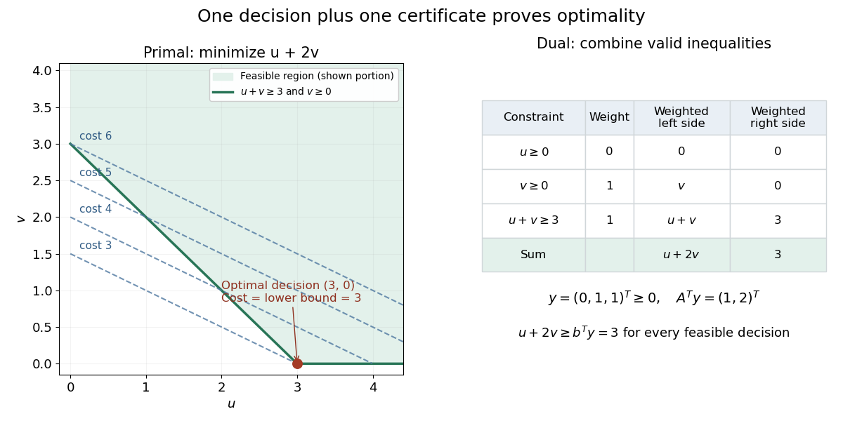
The entire dual feasible set can also be read off: write $y=(1-r,2-r,r{)}^T$ with $0\le r\le 1$. Then $A^{T}y=c$ and $b^{T}y=3r$. Maximizing this lower bound gives $r=1$. A point such as $r=1/2$ is still a valid certificate of the weaker bound $u+2v\ge 3/2$.

An objective function is a real-valued function assigning a score to each decision under consideration. An optimization problem seeks a feasible solution maximizing or minimizing this score. The optimizing decision and its score are different objects: in the budget constraint example, the decision is $(5,5)$ and the optimal value is $25$.

Choosing an objective function expresses what matters. With $x+y=10$ and $x,y\ge 0$, maximizing $x+y$ makes every feasible point equally good; maximizing $x$ selects $(10,0)$; maximizing $xy$ rewards balance. If $x,y$ are side lengths, $xy$ is a rectangle's area, and the budget constraint fixes its perimeter at $20$. The same mathematics then says that a square encloses the largest area among these rectangles.

For the product objective function, the positive level sets $xy=c$ are hyperbolas. Each collects decisions with identical scores. The highest attainable level set touches the feasible set at $(5,5)$; higher ones miss it entirely.

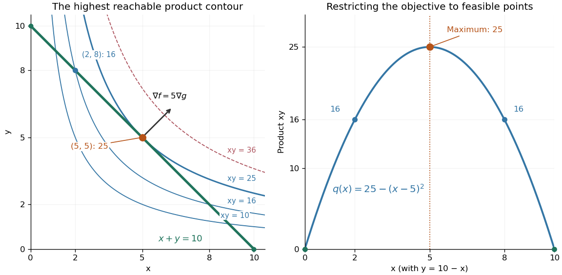
The product $xy$ is neither a convex function nor a concave function on the positive quadrant: along $(t,t)$ it is $t^2$, while along $(t,10-t)$ it is $10t-t^2$. Yet its restriction to this feasible set is a strictly concave function. Thus the geometry of the allowed decisions can make an otherwise nonconcave maximization problem tractable. Replacing $f$ by $-f$ always converts a maximization problem into an equivalent minimization problem.

// Target: mathematical-optimization.bigb

The objective function $\theta$ is nonnegative. We now construct a feasible zero-objective point, distinguishing the input problem's possible states.

If the primal is feasible and bounded below, strong duality and attainment for a linear program give $x_{\ast }\ge 0$, ${\lambda }_{\ast }$ and $s_{\ast }=c-A^T{\lambda }_{\ast }\ge 0$ withSet $\theta =\kappa =0$, $\tau =1$, $x=x_{\ast }$, $s=s_{\ast }$, $\lambda ={\lambda }_{\ast }$, andThe first three embedding equations hold. Substituting their equalities into the fourth gives precisely $-e^T{x}_{\ast }-e^T{s}_{\ast }-1+N\rho =0$.

If the primal is infeasible, the Farkas alternative supplies $\lambda$ with $A^T\lambda \le 0$ and $b^T\lambda >0$. Take $x=\tau =\theta =0$, $s=-A^T\lambda \ge 0$, $\kappa =b^T\lambda >0$, and $\rho =(e^{T}s+\kappa )/N$. These satisfy the same equations. If the primal is feasible and unbounded below, it has a direction in the recession cone $x\ge 0$ with $Ax=0$ and $c^{T}x<0$. Set $\lambda =s=\tau =\theta =0$, $\kappa =-c^{T}x>0$, and $\rho =(e^{T}x+\kappa )/N$. This is again a feasible nonzero embedding vector. Normalize the constructed vector by the sum of its nonnegative coordinates. In every case,The facts about optimal pairs and recession directions follow from the polyhedral alternatives of linear programming duality; they do not require knowing their values or witnesses to write the transformed coefficients.

To recover information from the transformed optimum, multiply the first three original embedding equations by ${\lambda }^T$, $x^T$, and $\tau$, respectively, and add. Their cross terms cancel; the fourth equation givesAt $\theta =0$, nonnegativity forces $x^{T}s=0$ and $\tau \kappa =0$. The equations also implyThus any normalized zero-objective point has $\rho >0$: if $\rho =0$, all these coordinates vanish, and then $q=\lambda =\theta =0$, contradicting normalization.

If $\tau >0$, division by $\tau$ gives a primal-feasible point $x/\tau$ and dual-feasible point $\lambda /\tau$ with equal objective function values; hence they are optimal. If $\kappa >0$, then $\tau =0$, $Ax=0$, $A^T\lambda =-s\le 0$, andTherefore either $b^T\lambda >0$ certifies primal infeasibility, or $c^{T}x<0$ is an improving recession direction certifying dual infeasibility and unboundedness whenever the primal is feasible. If only the latter certificate is obtained and primal feasibility is unknown, apply the same construction to the feasibility problem with objective function $c=0$; it gives either a feasible point or a direct primal infeasibility certificate.

A degenerate optimal point can have $\tau =\kappa =0$ and convey neither conclusion. Choose an optimum in the relative interior of the optimal face of a linear program. The explicit existence argument above gives a point of this face with $\tau +\kappa >0$. A nonnegative coordinate which is positive somewhere on a face of a convex set is positive throughout its relative interior, so the chosen point has $\tau +\kappa >0$ and can be decoded. The assertion follows because a small relative-interior displacement in the direction opposite a positive-coordinate point would otherwise make that coordinate negative. Equivalently one may obtain a maximum-support optimum; choosing an arbitrary degenerate boundary optimum is insufficient.

This reduction is useful because an interior-point method now has a known strictly feasible start, a compact standard simplex slice, and a known target objective function. Projective rescalings can recenter positive iterates, and the transformed problem supplies optimality or infeasibility information without a separate guessed optimum. Polynomial bit-complexity claims need rational data with a finite encoding length. The printed bound $U$ on arbitrary real coefficients by itself does not bound denominators or the size of nonzero determinants; it is not a substitute for that encoding assumption.

Let $x$ be an extreme point and consider its active constraints. Their row vectors span ${\mathbb{R}}^n$. Otherwise a nonzero vector $h$ is orthogonal to every active row. All inactive inequalities have strictly positive slack; since there are finitely many, a sufficiently small $\epsilon >0$ makes both $x+\epsilon h$ and $x-\epsilon h$ feasible. Their midpoint is $x$, contradicting extremality.

Choose $n$ independent active rows and write the corresponding equalities as $Bx=d$. The matrix $B$ has integer entries, so $\det B$ is a nonzero integer and $|\det B|\ge 1$. By Cramer's rule,where $B_j$ replaces column $j$ by $d$. Every entry of $B_j$ has absolute value at most $U$, even when $b$ is real. The determinant expansion has $n!$ terms, each with absolute value at most $U^n$. ThereforeThis proves the integer-matrix vertex coordinate bound; only the denominator determinant requires integrality.

For an exact finite-input ellipsoid method, the numerical data must have a specified encoding. In the standard model the input is the dimensions, the integer matrix and a rational right-hand side in binary, together with bounds derived from their encoding lengths. The vertex estimate above remains valid for arbitrary real $b$, but arbitrary unencoded reals do not by themselves specify an exact computational decision problem. Clear the rational row denominators to obtain an equivalent integer system, and let $V\ge 1$ bound the resulting integer coefficients and right-hand sides.

Two precautions make a feasibility account valid even for unbounded or lower-dimensional polyhedra. First, nonempty polyhedra need not have extreme points. Nevertheless they have a feasible point in the box $[-R,R{]}^n$ with $R=n!V^n$. To prove this feasible-point box bound for a polyhedron with lines, intersect the polyhedron with an orthant containing one feasible point. Minimize the sum of the signed coordinates in that orthant. Its nonempty sublevel sets are closed and bounded, so the minimum is attained. The compact minimum face has an extreme point, which is also extreme in the orthant intersection. Its active rows come from the integer system and signed coordinate inequalities, still bounded by $V$. Applying the proved vertex estimate gives the box bound. This is an existence argument; the algorithm need not enumerate all orthants.

Second, a nonempty feasible set can have zero ambient volume. Use a small uniform relaxation with a certified rational infeasibility gap, rather than stopping on volume alone. For the integer system $\tilde{A}x\ge \tilde{b}$, putThe normalized integer Farkas infeasibility gap says that if the system is empty there is a multiplier $y\ge 0$ with ${\tilde{A}}^{T}y=0$, $1^{T}y=1$ and ${\tilde{b}}^{T}y\ge 1/D$. Its bound follows by maximizing the certificate's value in the normalized multiplier polytope: a vertex has at most $n+1$ positive entries, and a determinant denominator bounded by $D$. Any point satisfying the relaxed inequalities would then give the contradictionThus relaxation preserves emptiness. If the original system is nonempty, take its point $x_0\in [-R,R{]}^n$. The bounded relaxed setcontains a Euclidean ball around $x_0$ of radius $\rho =\min (1/2,\eta /(nV))$: each row changes by at most $\sqrt{n}V\rho \le \eta$, and the expanded box leaves room for the ball. Hence $Q$ is either empty or has an explicit positive inner-volume bound. This is the full-dimensional relaxation of integer inequalities principle.

Start with a ball, viewed as an ellipsoid, centered at zero with radius $n(R+1)$, which contains the search box. At each iteration test its center against all inequalities defining $Q$. If the center is feasible, the preserved-emptiness result answers that the original problem is nonempty. Otherwise a violated row supplies a separation oracle cut. Move that cut parallel to itself through the current center if necessary, and compute a smaller containing ellipsoid for the surviving half. Every feasible point remains in the new ellipsoid.

The central-cut ellipsoid volume bound gives a shrinkage factor at most $e^{-1/(2(n+1))}$ for $n\ge 2$. After $O(n^2\log (n(R+1)/\rho ))$ cuts, the volume is below that of a radius-$\rho$ ball. If no feasible center has been found, $Q$ and therefore the original system are empty. Dimension one uses interval bisection. The logarithms of $R$, $D$ and $1/\rho$ are polynomial in the encoded input size. Standard outward-controlled finite-precision ellipsoid updates preserve enclosure with polynomial bit complexity.

The coordinate bound therefore supplies the initial bounded search region; the rational gap supplies a valid stopping threshold. Neither unboundedness nor zero volume of the original polyhedron can be ignored when deciding emptiness.

Introduce nonnegative slack variables $s_1,\dots ,s_4$ and write $z$ for the objective value. The initial simplex dictionary, recovered from the original PDF rather than the corrupted converted table, isFor this minimization convention, nonnegative objective coefficients give dual feasibility. The dual simplex algorithm repairs a negative basic value while retaining those nonnegative reduced costs. If the leaving row is $x_B=b+{\sum }_j{a}_j{x}_j$, $b<0$, an entering variable must have $a_j>0$; choose the smallest ratio of its objective coefficient to $a_j$.

Choose $s_1$ to leave. Eligible columns are $x_1,x_3$, with ratios $2/1=2$ and $18/6=3$. Thus $x_1$ enters. Solving its row and substituting givesNow only $s_3$ has a negative basic value. Its only eligible entering column is $x_3$, so pivot there, with $s_3$ leaving. The resulting dictionary isSetting the nonbasic variables $s_1,x_2,s_3$ to zero gives a basic feasible solution. The final objective row also proves $z\ge 23$ for every feasible point, because its nonbasic variables are nonnegative. Hence the unique relaxed optimum is

For the integer program, all four original slack variables are integers whenever the decision variables are integers. The fractional row can be writtenThe Gomory fractional cut keeps the fractional parts of these coefficients: $\{-1\}=\{-2\}=0$ and $\{-1/2\}=1/2$. It therefore gives $\frac{1}{2}{s}_3\ge \frac{1}{2}$, or $s_3\ge 1$. Its validity can also be seen directly: the displayed row makes $s_3$ an odd nonnegative integer. In original variables this cut is $2x_1+10x_3\le 18$.

Introduce the new integer-valued slack $u=s_3-1\ge 0$, with initial row $u=-1+s_3$. It is primal infeasible but retains dual feasibility, so one more dual-simplex pivot has $u$ leave and $s_3$ enter. Substitute $s_3=1+u$ to obtainAll basic values at $s_1=x_2=u=0$ are nonnegative integers, including $s_3=1$. The objective row proves a lower bound of $26$ on every point satisfying the valid cut, hence on every integer-feasible point. It is attained atThe strictly positive nonbasic objective coefficients also show uniqueness. One Gomory cut and its reoptimization are sufficient.

Assume $n\ge 1$ and the integer coefficient bound $U\ge 1$. There are $m(n+1)$ integers to record. Each signed integer in $[-U,U]$ can be encoded in $\lceil {\log }_2(2U+1)\rceil$ bits, so a fixed-width dense encoding needsbits, including the dimensions and bound. Its size is $\boxed{O(mn\log (U+1))}$. This is the bit-input model used for polynomial time; an arithmetic-operation count alone would not suffice.

We first construct a rational feasibility certificate for integer inequalities. Choose a feasible point and an orthant containing it, adding coordinate inequalities of the form $x_i\ge 0$ or $-x_i\ge 0$. The intersection $Q$ is nonempty. Starting at a point of $Q$, if the active constraint normals have rank less than $n$, choose a nonzero direction $d$ annihilating them. A sufficiently short move in either direction remains feasible, since every inactive constraint has positive slack. At least one direction has a finite endpoint: a nonzero coordinate of $d$ can be oriented toward the orthant boundary. Move to the first constraint met along such a direction. Its normal does not annihilate $d$, so it is independent of the previously active normals. Their rank strictly increases. In at most $n$ moves we obtain a point with $n$ independent active constraints.

At that point $Bx=d_0$ for an invertible integer $n\times n$ matrix $B$. Its rows are original constraint rows or signed coordinate rows, and $d_0$ has entries from $b$ or zero. All entries have absolute value at most $U$. By Cramer's rule,where $B_i$ replaces column $i$ by $d_0$. The Hadamard determinant inequality bounds both determinants by $(\sqrt{n}U{)}^n\le (nU{)}^n$. The denominator is a nonzero integer. Hence each coordinate has the claimed representation with numerator and denominator bounded in absolute value by $R=(nU{)}^n$. The orthant argument is needed because $P$ itself may contain lines and have no vertex. If $U=0$ is allowed literally, all coefficients and right sides vanish, and $x=0$ is feasible; the printed fraction bound then needs $U$ replaced by $\max (1,U)$, since a nonzero denominator cannot have absolute value at most zero. The bound just proved uses the customary positive coefficient bound.

Recording $n$ such fractions takes $O(n^2\log (nU))$ bits. A verifier checks that denominators are nonzero, changes their signs if needed, and verifies all inequalities by exact integer arithmetic after multiplying by positive denominators. The intermediate integers still have polynomial bit length. Thus a yes-instance has a polynomial-size, polynomial-time verifiable witness, and $\boxed{\mathrm{FP}\in \mathbf{NP}}$.

For optimization, let $c$ be rational with a finite binary encoding; clear its denominators to make it integer, which multiplies the objective by a positive constant and preserves its minimizers. All bit bounds below include the encoding length of $c$. Let $V=\max (1,{\max }_i|c_i|)$ and $B_0=nVR$.

A useful refinement of the preceding vertex argument is that if an objective is bounded below, a feasible point can be moved to an orthant vertex without increasing its objective. Choose the annihilating direction to have $c^{T}d\le 0$. If the inequality is strict, the forward feasible interval must have a finite endpoint, since otherwise the objective would be unbounded below. If $c^{T}d=0$, choose either finite endpoint supplied by the orthant. Rank increases as before. There are only finitely many such vertices across the finitely many orthants. Every feasible point therefore has one of these vertices with no larger objective; taking the least vertex value proves that a finite optimum is attained at one of them.

The Cramer representations at this optimum have one common denominator $\det B$, of magnitude at most $R$. Therefore its objective value $z^{\ast }$ has a representation with denominator at most $R$ and numerator at most $B_0$. In particular $|z^{\ast }|\le B_0$. No enumeration of orthants or vertices is part of the algorithm; they provide only polynomial-bit bounds.

Here is an exact linear optimization from a feasibility oracle. First call the assumed ellipsoid method feasibility routine on $P$; if it is empty, report infeasibility. Otherwise query feasibility with the extra inequality $c^{T}x\le -B_0-1$. A yes answer proves unboundedness below, because any finite optimum would be at least $-B_0$; an unbounded objective necessarily gives a yes answer. Thus the infeasible, unbounded and finite-optimum cases are distinguished using two feasibility calls.

In the finite case, maintain an infeasible lower threshold $-B_0-1$ and a feasible upper threshold $B_0$. Bisect the interval, querying $c^{T}x\le t$ each time. After polynomially many calls its length is less than $1/(2R^2)$, and $z^{\ast }$ lies in the resulting interval. Distinct reduced fractions with positive denominators at most $R$ differ by at least $1/R^2$, so there is only one possible value. It can be recovered in polynomial time by continued fractions: for the midpoint $t$, $|z^{\ast }-t|<1/(4R^2)\le 1/(2q^2)$, where $q\le R$ is the denominator of $z^{\ast }$. Thus $z^{\ast }$ occurs among the continued-fraction convergents of $t$. Compute those by the Euclidean algorithm and choose the unique fraction with denominator at most $R$ in the interval. If $t=z^{\ast }$, use the final exact convergent. The Euclidean algorithm and all thresholds have polynomial bit length.

Even if the feasibility routine returns only a decision, an optimal point can be recovered without assuming a witness-producing oracle. Add $c^{T}x=z^{\ast }$ and $-R\le x_i\le R$ for all $i$. This bounded optimal convex polytope is nonempty, since the optimal vertex above lies in it. Clear the denominator of $z^{\ast }$ and setAll vertex coordinates of this fixed convex polytope have denominators at most $D_0$ by the same determinant argument. Minimize $x_1$, recover its exact minimum by feasibility bisection and rational reconstruction, then fix it; do the same for $x_2$, and so on. Each restriction is an optimal face of the same original bounded convex polytope, so its vertices are original vertices. The single denominator bound $D_0$ therefore works at every step; repeated new precision bounds do not grow exponentially. After $n$ steps all coordinates are fixed to a feasible optimizer. There are polynomially many calls on polynomial-length rational instances, converted to integer inequalities by clearing denominators. Consequently linear optimization has a polynomial-time algorithm whenever linear feasibility does, with exact optimal value and optimizer, and correct reports of infeasibility or unboundedness.

The same relative coordinates give the proximity time of translating line segments asThis is a convex norm-constrained problem, rather than the linear feasibility problem for contact. One can solve it as a small second-order cone problem. If the distance between the initial line segments is at most $d$, the answer is zero; if no feasible point exists, the threshold is never reached.

For an elementary analytic algorithm, consider the nine combinations in which each of $s,r$ is either free, fixed at zero or fixed at one. In each case, minimize the squared distance over the free parameters. Writing $q(t)$ for $D+tv$ plus the fixed endpoint contributions, and $K$ for the columns belonging to free parameters, stationarity isIf the Gram matrix $K^{T}K$ is nonsingular, $z(t)=-(K^{T}K{)}^{-1}{K}^{T}q(t)$ is affine in time. Retain only the time interval on which its entries lie in $[0,1]$. The residual is then $r_0+t{r}_1$, and feasibility reduces toIntersect its solution interval with $t\ge 0$ and the free-parameter validity interval, and record the first point. Include the four endpoint–endpoint cases, where there are no unfixed segment parameters. Take the earliest valid candidate among all cases. The actual closest pair belongs to one of these faces of the parameter square, so this enumeration cannot miss the first approach.

The complications are the quadratic threshold equation, changes of the active closest-point feature and singular Gram matrices for parallel or degenerate segments. In a singular case, keep the affine family of minimizers and its feasibility bounds, or use the original convex problem; a pseudoinverse answer alone can fall outside the segment even when another minimizer is feasible. Constant-distance cases and tangential threshold contact must also be retained. Merely checking moving endpoints misses approaches between interior points.

Use payoff $P=-(2x_1-3x_2-2x_3)$, so maximization of $P$ is equivalent to the required minimization. In the given simplex tableau, $x_1$ can increase the payoff. The simplex ratio test has candidate ratios $3/6=1/2$ in the $z_2$ row and $15/1=15$ in the $z_3$ row; the negative coefficient in the $x_2$ row imposes no upper bound. Thus $x_1$ enters the simplex basis and $z_2$ leaves.

Divide the pivot row by $6$, then eliminate $x_1$ from the other rows. The resulting simplex dictionary isAll slack variables and original variables are nonnegative. The last row therefore proves $P\le 8$ for every feasible point; setting the nonbasic variables $x_3,z_1,z_2$ to zero attains it and leaves all basic variables nonnegative. HenceThe slack vector is $(0,0,29/2)$.

Fix a primal feasible point $x_0$. For every dual feasible point $y$, nonnegativity and the primal and dual inequalities giveHence the dual objective is bounded below by $c^T{x}_0$ wherever it is feasible, which is weak duality. This is the meaning of “bounded” in this assertion; it does not say that the dual feasible set is bounded, or that it is nonempty. For example, with $A=0$, $b=0$, $c=1$ and a single variable, the primal is feasible and unbounded above, while its dual would require $0\ge 1$ and is infeasible.

Let the finite primal supremum be $v$. First it is attained. The setis a finitely generated cone, hence closed by the argument in the root Solution. For a sequence of primal feasible points whose values approach $v$, the pairs $(b,c^{T}x)$ belong to $K$. Their limit $(b,v)$ therefore belongs to $K$. It gives a feasible point $x_{\ast }$ with $c^T{x}_{\ast }\ge v$, so necessarily $c^T{x}_{\ast }=v$.

Let $I$ index the tight primal inequalities at $x_{\ast }$ and let $Z$ index its zero coordinates. Consider the closed convex cone generated by $A_i^T$ for $i\in I$ and $-e_j$ for $j\in Z$. If $c$ were outside this cone, separation from a closed convex cone would give a direction $d$ withFor sufficiently small positive $\delta$, $x_{\ast }+\delta d$ remains a feasible point: the active constraints have the required signs, and every inactive constraint retains its positive slack. Its larger objective contradicts optimality. Therefore there are $y_i\ge 0$, supported on $I$, and ${\mu }_j\ge 0$, supported on $Z$, such thatThis makes $y$ a dual feasible point. Moreover, the support restrictions giveTogether with weak duality, this proves strong duality and dual attainment: