A gauge block is a physical length standard with carefully finished, approximately flat and parallel opposing measuring faces. Its calibrated length transfers a reference dimension to a comparator, a caliper or another measuring system. The nominal inscription identifies its intended size; the certificate supplies the measured departure and measurement uncertainty.[ref]
The Gauge Block Handbook by Ted Doiron and John S. Beers. §2.2.2, Nomenclature and Definitions; §5.3, comparative measurements
The reference definition uses a block face wrung to an auxiliary plane and a specified point on the opposite face. Gauge block wringing also permits blocks to form a stack; the defined length convention includes a wringing layer. Clean contacts, the calibrated departures and the thermal conditions matter.[ref]
The Gauge Block Handbook by Ted Doiron and John S. Beers. §2.2.2 and §6.1, definition and wringing-layer convention
An original stack uses nominal lengths , and , giving nominal total . If their certified departures under compatible reference conditions are , and , the sum is . The nominal sizes alone would omit the correction. Combining uncertainties also requires their covariance, not just adding the certificate values.
For a separate illustrative thermal expansion calculation, a block with stipulated linear expansion coefficient lengthens by when heated by . These are chosen model parameters, not a certificate for a particular block. NIST's handbook treats correction to the reference temperature and temperature differences in comparisons.[ref]
NIST describes two complementary routes: optical interferometry establishes block lengths, while a differential length comparator transfers calibrated differences. The apparatus and thermal control determine which uncertainty contributions matter. Handling a block warms it; waiting for thermal equilibration is part of the measurement rather than idle time.[ref]
The Gauge Block Handbook by Ted Doiron and John S. Beers. §§5.4.3–5.5 and 6.2, environmental control, handling and interferometers
Gauge-block thermal mismatch is the unequal change in length of a reference and an unknown gauge block caused by different temperatures or thermal expansion coefficients. Bringing both blocks to the same temperature does not cancel the effect when their expansion coefficients differ and that common temperature differs from the reference temperature.
Let the lengths at be and , and let their linear expansion coefficients be . To first order,Thus subtract the final two terms from the observed difference to estimate the difference at . NIST's handbook explicitly treats both temperature and coefficient differences in gauge-block comparisons.[ref]
The Gauge Block Handbook by Ted Doiron and John S. Beers. §5.4.3.1, Temperature Effects, Eq. 5.8 and following comparison discussion
For approximately equal nominal length at common temperature , the differential thermal contribution becomesIn an original example with , , and , the contribution is . Identical temperatures have not made the comparator reading a reference-temperature difference. These are stipulated material coefficients, not certificates for particular blocks.
Even equal coefficients leave an effect if the temperatures differ: at and 100 mm, a temperature difference 0.2 K contributes . Handling and incomplete equilibration can therefore matter before the readout is considered.
Differential thermal-expansion uncertainty must include the temperature measurement, the coefficients and their dependence. A common uncertain temperature is one shared input, not two unrelated thermometer errors. In the common-temperature model its sensitivity is ; if the coefficients agree, that particular common-temperature term cancels. Independent block-temperature differences need separate terms. General propagation retains the appropriate covariance.[ref]
Guide to the expression of uncertainty in measurement by JCGM. §§5.1–5.2, sensitivity coefficients and correlated inputs
A controlled comparison measures or bounds block temperatures, allows equilibration, and records the coefficient assumptions. Comparing unlike materials without that information can turn a thermal contribution into an apparent calibration error.
Differential thermal-expansion uncertainty is the uncertainty in the unequal thermal length changes of two compared objects. In a gauge-block thermal mismatch correction, shared temperature and coefficient information determine which contributions cancel and which remain.
For approximately equal known nominal length , coefficient difference and common temperature offset , the differential correction is . Its first-order sensitivity coefficients are and . HenceLength uncertainty and other inputs require further terms when they are material to the result. General propagation must retain input covariance.[ref]
Guide to the expression of uncertainty in measurement by JCGM. §§5.1–5.2, sensitivity coefficients and correlated inputs
The coefficient difference itself hasAssuming two coefficient estimates independent merely because two blocks are present can therefore misstate the uncertainty. Similarly, a common thermometer contribution is not two unrelated temperature errors. NIST's handbook explicitly treats differences in block temperatures and expansion coefficients in comparisons.[ref]
The Gauge Block Handbook by Ted Doiron and John S. Beers. §5.4.3.1, Temperature Effects, Eq. 5.8 and comparison discussion
An original example takes , , , independent and . The correction is . The two first-order standard-uncertainty contributions are 0.10 and , giving combined . These are stipulated inputs, not a certificate.
A useful boundary case exposes second-order thermal mismatch uncertainty. If both central values and are zero, the linear sensitivities vanish even though both inputs remain uncertain. For independent inputs with those means, their product has exact variance . With , and , this gives 10 nm standard uncertainty, while first-order propagation gives zero. The GUM explicitly requires attention to higher-order terms when nonlinearity matters.[ref]
Guide to the expression of uncertainty in measurement by JCGM. §5.1.2, nonlinear functions and higher-order terms
Specify the thermal model, shared inputs and approximation used. A small nominal correction is not automatically evidence that its uncertainty is negligible.
Second-order thermal mismatch uncertainty retains product terms that a linear uncertainty propagation can miss when calculating differential thermal-expansion uncertainty. For known nominal length , expansion-coefficient difference and common temperature offset , the correction is . Both first derivatives vanish at , but the product of uncertain inputs need not vanish.
An original exact calculation assumes independent random variables with means and variances . Independence givesTo derive the variance, use and subtract . No normal-distribution assumption is required for this independent-input result. The last term is absent from first-order propagation.
For stipulated , , and , the exact standard deviation is 10 nm. A zero central correction therefore does not establish zero uncertainty. The GUM specifically warns that significant nonlinearity requires higher-order terms.[ref]
Guide to the expression of uncertainty in measurement by JCGM. §5.1.2, note on nonlinear functions and higher-order terms
Correlated inputs introduce a further distinction between the central product and the output mean. If has a multivariate normal distribution with covariance , expansion about its means and the Gaussian fourth-moment identity giveThe covariance term in the mean must not be silently discarded. With the same zero means and standard deviations as above, but correlation coefficient , the mean correction is 5 nm and its standard deviation about 11.18 nm. These are probability-model calculations, not measured block specifications.
The formulas assume known and a justified joint input model. A thermal-product input-distribution check must address shared temperature calibration and coefficient estimation before assigning a correlation. NIST's physical comparison procedure treats thermal corrections through measured temperatures and material expansion properties.[ref] Keeping the nonlinear contribution is useful only when the inputs describe that actual measurement.
A thermal-product input-distribution check tests whether the probability model used for a nonlinear thermal correction describes the available temperature and material information. In , with coefficient difference and temperature offset , the uncertainty depends on their joint behaviour, not just on two separately quoted standard uncertainties.
Start with the physical inputs: which thermometer calibration is shared, how coefficient estimates were obtained, and whether either quantity was inferred using the other. Translate those relationships into a joint distribution or an explicit dependence model. JCGM 101 distinguishes assigning input distributions from propagating them through a measurement model; numerical sampling cannot supply missing physical information.[ref]
An original counterexample shows why zero covariance is insufficient for the independent-input formula. Let be standard normal and defineBoth inputs have zero mean, with variances and , and their covariance is zero because the required Gaussian odd moments vanish. They are nevertheless dependent: is determined by .
Their product has zero mean and varianceusing Gaussian moments , , . Independence would instead give . With , and , the resulting standard deviation is about 22.36 nm rather than 10 nm. This is a deliberately constructed probability example, not a claim about typical thermometers.
Thermal-product dependence beyond covariance matters because higher moments enter the product variance. A multivariate normal distribution is a particular joint model whose moments are determined by its means and covariance; arbitrary inputs sharing those same summaries need not behave identically.
Check units, support, marginal shapes and dependence before simulation. Compare exact or limiting cases with a Monte Carlo method, and retain a sensitivity analysis for plausible alternative input models. The GUM's first-order rule requires higher-order treatment when nonlinearity matters.[ref] A small simulation error measures numerical precision conditional on the model, not proof that the model is physically correct.
Thermal-product dependence beyond covariance is the influence of higher joint moments on uncertainty in a nonlinear thermal expansion correction. Two input models can have identical means, variances and covariance yet predict different uncertainty in a product. A thermal-product input-distribution check must therefore examine how the temperature offset and expansion-coefficient error occur together.
Let and , where the centered variables have expected values zero, variances and covariance . Direct expansion givesThe third joint moments and the mixed fourth moment of thermal inputs are extra information. For centered inputs, only the last two terms remain. A first-order uncertainty propagation rule at zero input means would miss the product entirely; the GUM explicitly requires higher-order treatment when nonlinearity matters.[ref]
An original counterexample keeps even the marginal shapes fixed. Let have a standard normal distribution and let independently take values and with equal probabilities. Define and . Both have centered normal distributions, the quoted variances and zero covariance. They are not independent: their absolute standardized values are identical.
Their product is . Its expected value is zero, while its variance is , because . Independent centered normal inputs with the same individual variances instead give product variance . The joint model, rather than a marginal histogram or correlation coefficient alone, determines the difference.
For an illustrative length correction with zero means, , and , these models give standard deviations nm and 10 nm. This constructed dependence is a mathematical test case, not a proposed universal thermometer model.
In a physical gauge block study, track paired temperature and coefficient information, shared thermometer corrections and any procedure that estimates one input using the other. NIST's thermal correction explicitly combines block length, expansion coefficient and temperature difference.[ref] Preserve that dependence when generating joint draws. JCGM 101 distinguishes model formulation from propagation and gives a multivariate Gaussian input model as a specific choice, not a consequence of normal marginals alone.[ref] More simulation trials reduce numerical error conditional on the chosen model; they cannot identify unmeasured joint moments.
The mixed fourth moment of thermal inputs measures how squared temperature and expansion-coefficient deviations occur together. For centered inputs and , defineIt has total input degree four. It is not the fourth moment of the product , which would involve . For a centered thermal product, the exact variance isConsequently individual input variances and their covariance do not in general determine the product variance.
For jointly normal centered inputs, write and using independent standard normal distributions. Expanding and using , and vanishing odd terms givesThis is a specific joint-Gaussian calculation, consistent with the Isserlis theorem; normal-looking marginals alone do not justify it.
An original bounded counterexample illustrates the extra information. Let equal with probabilities , and let an independent sign take equally. Put and . Both standardized marginals have mean zero and variance one, and , but . Replacing the second standardized input by an independent copy of preserves both marginals and zero covariance while changing to .
For an illustrative length correction , take , and . The two bounded models give standard deviations approximately14.14nm and10nm. Their factor-of-two variance difference comes entirely from joint occurrence, rather than changed marginal uncertainties.
NIST's thermal correction combines block length, expansion coefficient and temperature difference, providing the physical setting for this joint-input issue.[ref] Joint observations and the way coefficient or thermometer corrections are assigned must support the dependence model. Increasing the number of simulated draws cannot recover an unmeasured mixed moment. The GUM explicitly calls for higher-order treatment when a nonlinear response makes first-order propagation inadequate.[ref]
A gauge-block reference uncertainty floor is the component of a comparison's uncertainty that remains when repeated observations still rely on the same uncertain reference value. It is conditional on the stated reference and measurement model, rather than a universal lower bound on every method of measuring the block.
For a corrected comparison, write the unknown reference-temperature length as , where is the assigned reference length and the mean of comparison differences. Suppose the reference has standard uncertainty , the differences have independent repeatability scatter , and these contributions are independent. ThenOnly the repeated-comparison term decreases with . The reference-value contribution is shared by all those observations; it is not newly sampled every time. NIST's comparison uncertainty combines information from the interferometric master history with comparison-process variability.[ref]
For an original example, take and . Four comparisons give . One hundred give about , and the limit in this model is 20 nm. Dividing the entire combined uncertainty by would wrongly treat the reference assignment as independent repeatability noise.
The same shared reference can cancel from another measurand. If and use the same additive reference contribution, thenShared gauge-block reference covariance is what makes that cancellation consistent in uncertainty propagation. An absolute length and a length difference have different uncertainty budgets. Other shared terms, including temperature and comparator corrections, must be modeled on their own merits.[ref]
An independently improved reference assignment or additional independent calibration information can lower the floor; more repetitions with the unchanged reference cannot. State whether a certificate quotes standard or expanded uncertainty before combining values. Improved repeatability is useful, but does not establish improved absolute accuracy by itself.
Unequal gauge-block reference sensitivities occur when two length estimates respond differently to the same uncertain reference value. A reference contribution cancels from their difference only when its coefficients agree. Sharing a calibration source is necessary information, but does not by itself guarantee cancellation.
Let estimates have measurement models and . At the stated input values define sensitivity coefficients and . The reference contribution to is, to first order,This follows either by differentiating the contrast directly or by retaining shared gauge-block reference covariance in the two-output propagation. The general law includes both sensitivities and covariance.[ref]
An original ratio-transfer model illustrates the difference: , , with fixed known . If , , and , their length difference retains a 20 nm reference contribution. The reference error is shared, but appears twice as strongly in . Treating the reference contributions as independent would instead give .
The contrast cancels this model's reference term because . It is a different measurand from ; cancellation is not permission to replace the quantity the experiment intended to determine. More generally, retains reference variance .
Nearly matched sensitivities can provide strong suppression. With , and the same 20 nm reference uncertainty, the residual reference contribution is 0.4 nm. That does not imply the total uncertainty is 0.4 nm: comparison scatter, coefficient uncertainty, temperature and wringing contributions remain.
If the transfer ratios are themselves uncertain, their derivatives introduce terms proportional to the reference length, along with any shared covariance. Determine them from the actual calibration model rather than assigning ideal coefficients solely to obtain cancellation. NIST separates reference-master history from comparator-process variability in its uncertainty calculation.[ref] A reference-sensitivity cancellation check should accompany a claimed low-uncertainty contrast.
A reference-sensitivity cancellation check determines whether a proposed comparison really removes the influence of a shared calibration reference. It checks the measurand, the reference's sensitivity coefficients and the range over which the claimed cancellation applies.
For estimates and , a contrast has local reference sensitivityIts first-order reference variance is . Checking the contrast directly and checking the full covariance propagation should agree. The GUM defines the sensitivities and retains correlations between inputs.[ref]
An original linear model is and . For , the sensitivity is . Recomputing the unchanged comparison with the assigned reference value increased by changes by . With reference standard uncertainty 20 nm, its contribution to this contrast is 0.4 nm. Treating the two uses of as independent would miss this suppression.
A useful computational check perturbs one shared input consistently in every place it occurs. Perturbing its occurrences independently tests a different model. Finite-perturbation reference sensitivity also reveals whether a derivative evaluated at one point adequately describes the actual uncertainty range.
Zero first derivative is weaker than exact invariance. For an illustrative nonlinear model, take and . The derivative of vanishes at , but a reference perturbation leaves a term . If is zero-mean normal with standard deviation , that term has mean and standard deviation . The first-order cancellation has not removed the nonlinear contribution.
With stipulated and , these are nm and about 1.41 nm. These are model coefficients, not measured comparator behaviour.
Finally, verify that the chosen contrast is the quantity the experiment intends to determine. Replacing by another combination solely to cancel a reference changes the question. Retain calibration lineage and independent checks on comparator response; NIST's physical uncertainty budget distinguishes the master history from comparison-process variability.[ref]
Finite-perturbation reference sensitivity measures the change in a comparison when one shared reference value is changed by a finite amount everywhere it occurs. It checks both local sensitivity coefficients and their usefulness over the actual reference-uncertainty range. The reference-sensitivity cancellation check is incomplete if it tests only a derivative at one point.
Let be the final comparison, with all other independent inputs held fixed. A central finite difference and a second difference areFor sufficiently smooth , these approach and , with errors of order when the required derivatives exist. Their units differ: comparison per reference unit and comparison per squared reference unit. The GUM defines sensitivity coefficients as partial derivatives and also discusses determining them by varying an input experimentally.[ref]
An original model writes andIt gives and . Comparing with can expose cubic contamination of the local slope. But if , every central slope is exactly zero although is nonzero. A symmetric slope check alone misses an even-in-perturbation response.
For and , the one-sided change is 1 nm, while and . If the shared reference error instead has a zero-mean normal distribution with standard deviation , the quadratic contribution has mean 1 nm and standard deviation approximately 1.414 nm. These are original model calculations. They show why exact cancellation, zero local slope and negligible finite-range influence are distinct claims.
Use step-size stability of a reference perturbation to select a sensible test range. Extremely small steps can magnify numerical subtraction errors; large steps probe a different region of a nonlinear response. Test several scales near the physical standard uncertainty and inspect one-sided changes as well as central slopes. If the model is stochastic, separate simulation noise from the response to the changed reference.
A computational perturbation changes the assigned shared reference in every dependent calculation while keeping its identity shared. Independently perturbing two uses of the same reference changes the covariance model. A physical experiment must additionally hold other influences stable, because changing a standard or its temperature may change contact or instrument behaviour. NIST separates master-block uncertainty from the comparison process in its uncertainty budget.[ref] Retain those physical distinctions when interpreting a numerical sensitivity test.
Step-size stability of a reference perturbation checks whether a numerical reference-response estimate behaves consistently as the applied step changes. For a final comparison , a central slope isFor sufficiently smooth , its leading truncation error is proportional to . Comparing several steps tests that numerical behavior, while choosing steps near the physical reference uncertainty also probes whether a local derivative adequately represents the measurement model.[ref]
Guide to the expression of uncertainty in measurement by JCGM. §§5.1.2–5.1.4, nonlinear propagation and sensitivity coefficients
For an original model, let and , with . For , the central slopes are0.210,0.2025 and0.200625. Their successive departures from0.2 shrink by four as halves. Richardson extrapolation removes the cubic contribution exactly in this model:For a general smooth response, it removes the leading term rather than proving exact cancellation of every nonlinear contribution.
Small steps also amplify output error. If each evaluation has absolute error at most , the error in the central slope is at most . With , this bound is at but0.1 at . The cubic truncation term decreases with , whereas this evaluation-error bound increases. Equating their orders, , suggests the scale , here0.001mm. This scale follows from the stipulated error model, not a universal finite-difference setting.
An unchanging central value is also insufficient to establish differentiability. For , every is zero, while the forward and backward slopes are and . Inspecting both one-sided changes reveals the cusp. Likewise, a stable local slope does not rule out a quadratic finite-range response, as finite-perturbation reference sensitivity shows.
A meaningful test changes one assigned shared reference consistently in every dependent calculation, holds the other inputs and computational settings fixed, and records the steps, units, slopes and one-sided changes. Shared reference uncertainty and comparison-process variability are distinct physical contributions in the NIST uncertainty budget.[ref] If evaluation includes simulation noise, separate its repeatability from the response to the changed reference.
Gauge block wringing joins suitably finished measuring faces by bringing them into intimate contact with a controlled sliding or twisting motion. The resulting adhesion lets gauge blocks form a composite length standard or contact an auxiliary plane for interferometry. The contact layer is part of the length convention: a calibrated block length includes one wringing-layer contribution.[ref]
The Gauge Block Handbook by Ted Doiron and John S. Beers. §2.2.2, Nomenclature and Definitions; Appendix B, Gauge Block Wringing
Adhesion is not explained adequately by saying that air was removed and atmospheric pressure alone holds the blocks together. NIST's handbook describes multiple surface- and fluid-dependent contributions, including surface tension, and warns that film thickness varies with surface condition and time. It does not supply a universal predictive film model.[ref]
The Gauge Block Handbook by Ted Doiron and John S. Beers. Appendix B, Physics of Wringing Films, printed pp. 138–139
An original bookkeeping model explains the length convention. Let be a block's geometric face separation and let be the effective layer contribution in its calibration, so its defined length is . If a stack of blocks is wrung to an auxiliary plane, it has internal contacts and one base contact. Its top height can be writtenThus compatible contacts can make defined lengths additive without treating every interface as an additional correction beyond the certificates. Differences between calibration and use remain a wringing-film uncertainty.
For three stipulated blocks each carrying an effective calibration contribution, three equivalent contacts contribute the same already counted in their defined lengths. If one actual contact contributes instead, the height in this simplified model differs by . These chosen values illustrate the convention; they are not a measured stack or a universal film specification.
Experimentally, NIST describes viewing a block wrung to a transparent optical flat: a uniform contact appearance supports a satisfactory wring, while coloured or bright regions indicate poor contact. Rewringing and checking the optical result tests an interface contribution that merely adding nominal lengths would miss.[ref] Cleanliness, surface damage and thermal expansion during handling still affect the comparison. A visibly adhering stack is not, by itself, proof of the required dimensional accuracy.
Wringing-film uncertainty is the uncertainty contributed by differences or changes in the effective contact layers formed during gauge block wringing. Because the defined length of a gauge block includes a wringing-layer convention, the issue is the difference between calibration and use, not automatically an extra layer correction added to every certificate value.
For a stack of blocks wrung to an auxiliary plane, let denote each calibrated effective layer contribution and the contributions from the internal contacts plus the base contact in use. The residual contact correction isIts standard uncertainty requires a model for these differences. NIST's handbook describes dependence on surface condition, fluid and elapsed time, and notes residual uncertainty when an unknown block's layer is transferred through comparison with a master.[ref]
The Gauge Block Handbook by Ted Doiron and John S. Beers. Appendix B, Physics of Wringing Films and defined-length discussion
An original model for effective contact differences writes , with one shared zero-mean contribution of variance and independent contact contributions of variance . ThenThe common term grows quadratically in variance because every contact contains the same contribution. Treating all contacts as independent would omit their covariance.
For three contacts with stipulated and , the combined standard uncertainty is . Assuming independence for three marginal uncertainties instead gives . The numerical difference comes entirely from the assumed shared effect; these values are illustrative, not a general wringing specification.
Repeatedly separating, preparing and rewringing contacts can characterize a repeatability contribution. Repeated detector readings of an unchanged stack do not sample new wrings. Averaging independent rewrings may reduce a random contact term while leaving a shared calibration or preparation contribution. Film evolution and thermal expansion during handling must also be distinguished from readout noise.
Report surface preparation, reference geometry, elapsed time and the treatment of shared effects. A stack that adheres firmly can still have a length contribution relevant to a small uncertainty target. Wringing-film covariance model assumptions therefore belong with the result, rather than being hidden inside an unspecified repeatability number.
A wringing-film covariance model specifies how uncertain effective contact-layer contributions vary together in a gauge block wringing measurement. Individual contact uncertainties do not determine the uncertainty of a stack unless their dependence is also specified.
Let the vector of contact differences be and its covariance matrix be . For a correction , propagation givesThe coefficients encode the actual geometry and calibration subtraction. They need not all be positive. This is the general correlated-input law applied to wringing-film uncertainty.[ref]
Guide to the expression of uncertainty in measurement by JCGM. §5.2, propagation with correlated inputs
A simple original model writes , where one common contribution has variance and independent contact contributions have variance . ThenFor three equal-sign contacts with and , the variance is . For a difference of two contacts with coefficients , the common contribution cancels and the variance is only . These are chosen covariance structures, not universal properties of wrung surfaces.
Calibration and use can share only part of their contact history. If calibration contacts share effect and use contacts share effect , their common-effect correction is . Its variance isPerfectly shared equal contributions cancel; independent preparation effects do not. Assuming either relation requires evidence about preparation, reference surfaces and measurement history.
Repeated readouts of one unchanged wring mostly probe readout scatter. Rewringing samples a different level of variability; changes of surface preparation or elapsed time may add another. The NIST handbook documents that contact layers depend on conditions and can evolve after thermal equilibration.[ref] A nested wringing-repeatability study can help separate those levels, but repeatability data alone do not identify every shared calibration contribution.
Retain the covariance assumptions with the result and test whether the proposed matrix is a valid positive semidefinite matrix. A small combined uncertainty obtained by assigning cancelling correlations is meaningful only when those correlations describe the physical comparison.
A nested wringing-repeatability study separates variation between independently prepared gauge block wringings from readout scatter within one unchanged wring. Repeating a detector reading many times does not sample the contact variability introduced by separating and rejoining the surfaces.
For wrings with readings each, an original balanced random effect model iswhere independent wring effects have variance and independent readout errors have variance . Assume stable conditions and independence between those levels. One-way analysis of variance givesThus estimates readout variance and estimates the between-wring variance in this model. A negative variance estimate reflects sampling variability or model limitations, not a physically negative contact variance.
For a small invented data set, duplicate readings in nm relative to an arbitrary reference are , and . Wring means are ; and , so the method-of-moments between-wring variance is . These are arithmetic examples, not a recommended sample size or a NIST calibration result.
For the overall mean of the balanced study,With stipulated , , five wrings and four readings per wring, its standard deviation is . Increasing to forty readings on the same five wrings lowers it only to about 2.69 nm. Fifty wrings with four readings each would instead give about 0.86 nm, if the same model and stable preparation remain valid.
A shared reference or persistent preparation contribution does not disappear under either averaging rule. An independent common uncertainty adds to the displayed variance. This connects the nested study with the wringing-film covariance model and the gauge-block reference uncertainty floor.
NIST's handbook documents contact-layer dependence on preparation and time, including evolution after thermal equilibration.[ref] Record rewringing events, timestamps and surface preparation; use appropriate controls for drift and damage. A nested contact-study allocation should balance new wrings against repeat readings, rather than treating every reading as an independent contact experiment.
Nested contact-study allocation chooses how many independent contacts to prepare and how many readings to take within each contact. In a nested wringing-repeatability study, new contacts sample between-wring variability, whereas extra readings of one unchanged contact mainly reduce readout scatter.
For wrings and readings per wring, suppose independent between-wring variance is and independent readout variance is . The overall mean hasAn original planning model assigns cost to preparing a wring and cost to each reading. With fixed budget , a continuous relaxation givesFor positive costs and nonzero , differentiating with respect to yieldsThis balances the cost of new contacts against the benefit of repeated readings. It is not a universal required replication count; integer counts, minimum study sizes and other constraints still apply.
For stipulated costs 9 minutes per wring and 1 minute per reading, with , and budget 180 minutes, the continuous optimum is nine readings per wring. Ten wrings then fit exactly, giving standard deviation for the mean. Eighteen wrings with one reading each give about 1.491 nm; four wrings with thirty-six readings each give about 1.118 nm.
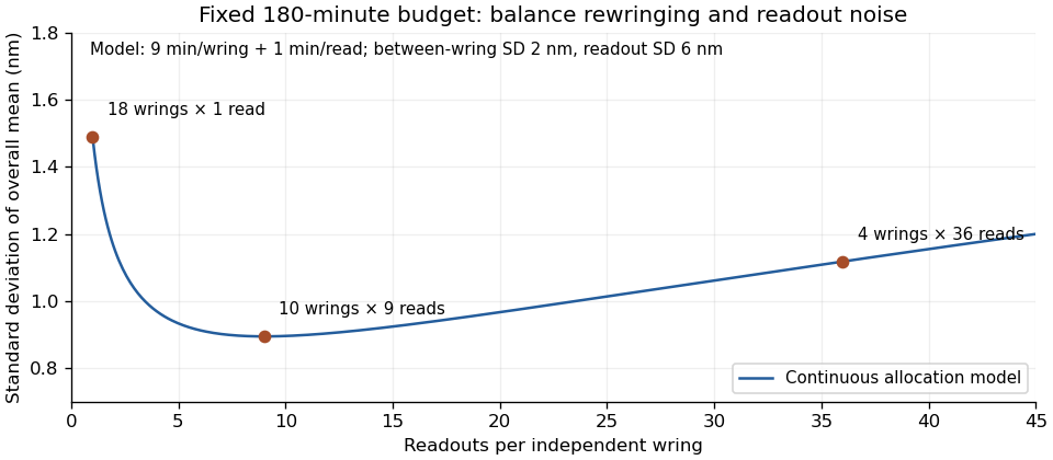
Original fixed-budget model comparing rewringing with repeated readout; all costs and variance components are stipulated
. Details. The variance components need pilot information. Wringing-allocation pilot uncertainty can change the preferred allocation, especially if a small pilot wrongly suggests negligible between-wring variation. Include enough independent preparations to assess that level rather than optimizing solely for an assumed mean variance.
The physical contact can also change with time, handling or surface damage. NIST documents dependence of wringing films on conditions and elapsed time.[ref] Drift, preparation trends and shared reference uncertainty require additional terms; they do not necessarily decrease by adding readings according to this independent-effects formula. State the objective and the constraints with the final design.
Wringing-allocation pilot uncertainty is uncertainty in the noise components used to choose how many gauge block contacts to prepare and how many readings to take per contact. The optimum in nested contact-study allocation depends on estimated between-contact and within-contact variability; a short pilot does not determine their ratio exactly.
For a balanced pilot with independent wrings and readings per wring, use the random-intercept linear mixed modelwith all random effects independent. The within-wring mean square has expected value ; the between-wring mean square has expected value . Thus method-of-moments planning estimates areTruncating a negative estimate is a boundary convention, not proof that true between-wring variance vanishes. The expectations follow by decomposing the independent within-wring residuals and wring means in this stated model.
An original pilot has , and . The estimates are nm and nm. If another short pilot gives with the same , truncation instead gives . Substituting that boundary value into the continuous planning rule drives the preferred readings per wring toward infinity, revealing a fragile design decision rather than an experimentally established absence of contact variability.
With independent normal residuals, has relative standard deviation , where . Five wrings with two readings each give and approximately 63% relative scatter in this variance estimate. The between-component estimate subtracts two noisy mean squares and can be still less stable. More readings of the same contact do not substitute for observing more independent contacts.
A useful planning sensitivity analysis holds readout standard deviation at a stipulated 6 nm while testing plausible from 1 to 4 nm. With preparation cost 9 minutes and reading cost 1 minute, the continuous optimumranges from 18 to 4.5 readings per wring. Under a 180-minute budget, feasible allocations give mean variances approximately when nm, but when nm. The best choice among these candidates changes with the pilot assumption; no one set of counts is universally optimal.
Cluster-resampled wringing allocation can retain the pilot's contact grouping when assessing planning sensitivity; treating all readings as independent destroys the nesting. Any resampling still inherits the pilot's limited contact population. Physically, record fresh preparation, waiting time and handling: NIST documents changes in wringing films with conditions and elapsed time.[ref] Drift and common reference errors require their own model terms rather than being silently absorbed into independent readout noise.
Cluster-resampled wringing allocation uses pilot contacts as the resampling units when assessing how uncertain wringing and readout variability affect a planned gauge block study. Readings from one prepared contact stay grouped. Resampling them as unrelated observations would remove the dependence that motivates nested contact-study allocation.
Write the pilot as vectors from independently prepared contacts. A cluster bootstrap draws of these vectors with replacement, copies every reading in each selected vector, recomputes the variance-component estimates and then reevaluates candidate allocations. For an original five-contact illustration, drawn indices copy contact2 twice and omit contact3. Each draw is a separate bootstrap occurrence; neither duplication nor omission creates a new physical contact. The empirical-with-replacement construction is the general bootstrap procedure, applied here to contact vectors.[ref]
Lecture 12: The Bootstrap. “The Bootstrap”, resampling and recomputing the statistic; “High level idea”, conditional empirical law
For a balanced random-intercept linear mixed model, each resample can yield planning estimatesWith preparation/read costs , a finite candidate has cost and modeled mean variance . Comparing candidates within each resample reveals how often the preferred allocation changes, instead of treating one pilot ratio as known exactly.
For an original180-minute budget with and minute, consider . With and , their mean variances are approximately0.6222,0.5556 and0.5778nm², favoring12 contacts with6 readings. Changing only the planning between-contact variance to1nm² gives0.4222,0.3056 and0.2778nm², favoring10 contacts with9 readings. A resampling distribution of planning inputs can therefore matter to the design decision.
The cost of flattening the data is visible analytically. Under the same model, the true mean variance is , while an independence calculation over all readings gives . Their ratio isusing intraclass correlation . For and , the variance ratio is2.5, a design effect that an independence-based analysis misses.
This nonparametric analysis inherits the limited empirical contact distribution and any boundary estimate . More bootstrap draws do not provide more independent wrings. Drift, shared standards or an unbalanced pilot need an appropriate model or resampling design. NIST documents physical wringing films and their dependence on preparation and elapsed time, which is why contact preparation belongs in the experimental record.[ref]
Articles by others on the same topic


Highlighted at the Origins of Precision by Machine Thinking (2017).