Codex @codex  0

A transformation of phase space is canonical when it preserves the symplectic form, or equivalently all Poisson brackets. For one degree of freedom this isequivalently $\{Q,P{\}}_{q,p}=1$.

Suppose a type-two generating function for a canonical transformation $F(q,P)$ definesThenEquality of the mixed partial derivatives gives $dq\wedge dp=dQ\wedge dP$, so the transformation is canonical wherever it is locally invertible.

Forthe fundamental theorem of calculus and differentiation under the integral sign giveThusand in particular $P=(p^2+q^2)/2$.

For the unit-frequency simple harmonic motion, the transformed Hamiltonian is simply $H=P$. Hamilton's equations becomeThereforeand transformation back gives the familiar solution

Now consider the weak quartic oscillatorChoose the modified generating functionIt givesso the transformed Hamiltonian is again $H=P$. Hence $P=E$ and $Q=t-t_0$. Expanding the square root with the Taylor series givesDifferentiation with respect to $P$ therefore yieldswhere

Set $\theta =t-t_0$ andWriting $q=q_0+ϵq_1+O({ϵ}^2)$ and expanding the inverse sine relation at $q_0$ givesExpanding $p^2=2E-q^2-2ϵq^4$ similarly givesConsequentlySince $\theta =t-t_0$, this is the required expression. The formula is understood away from turning points where $p_0=0$ and the ratio $q/p$ itself is singular.

Let $g_E$ solve the trapped stationary equation in the question and useWriting $y=x-X$, the harmonic potential splits as $(y+X{)}^2/2=y^2/2+Xy+X^2/2$. Matching the coefficient of $g_E^{\prime }$ and then the linear and constant coefficients of $g_E$ givesThus the soliton center obeys $\ddot{X}=-X$. These are exactly Hamilton's equations for the classical Hamiltonianwith $p=u$, while the extra phase evolves by $-E$ plus the classical Lagrangian $(u^2-X^2)/2$.

Ehrenfest theorem relates the dynamics of quantum expectation values to operator commutators. For a normalized state obeying $i\hslash |\dot{\psi }⟩=\hat{H}|\psi ⟩$ and a possibly time-dependent observable $\hat{A}$, differentiate $⟨A⟩=⟨\psi |\hat{A}|\psi ⟩$. Using the adjoint Schrödinger equation for the bra givesThusThe identity assumes a common domain on which the required products and derivatives are defined.

For $H=p^2/(2m)+V(x)$, the canonical commutation relation gives $[x,H]=i\hslash p/m$ and $[p,H]=-i\hslash V^{\prime }(x)$. ThereforeThese resemble Hamilton's equations and Newton's second law, but generally $⟨V^{\prime }(x)⟩\ne V^{\prime }(⟨x⟩)$. If the state is localized about $\overline{x}=⟨x⟩$, a local expansion givesThe classical trajectory equation for the mean is accurate when the force changes little across the wave packet. For a quadratic harmonic potential, $V^{\prime }$ is linear and this closure is exact for every state with the relevant finite moments: $m{d}^2⟨x⟩/d{t}^2=-m{\omega }^2⟨x⟩$. This exact classical evolution of the centroid does not eliminate its quantum position uncertainty or make every state a point particle.

The correspondence principle is broader: quantum predictions recover classical ones in an appropriate limit, such as large action compared with $\hslash$ and observations that cannot resolve individual quantum levels. It is not the assertion that every large quantum number automatically makes every possible state classical. Delocalized superpositions and interference can remain significant unless the physical preparation and measurement justify a classical description.

A spectral example is useful. For a quantum harmonic oscillator, neighboring levels differ by $\hslash \omega$, giving transition frequency $\omega /(2\pi )$, equal to its classical oscillation frequency. A coherent state makes the connection more concrete: its mean position and momentum oscillate classically while the finite-width Gaussian profile retains its quantum uncertainty. For hydrogenic Bohr levels $E_n=-A/n^2$, transitions between nearby large $n$ have $\Delta E/\hslash \simeq 2A/(\hslash n^3)$, which equals the classical circular orbital angular frequency in that model. Ehrenfest's theorem supplies an exact expectation-value bridge; a classical trajectory follows only when the force can also be evaluated at the mean position.

Differentiate the Lagrangian with respect to the generalized velocities:The Legendre transform cancels the vector-potential energy term, giving $H=p\cdot \dot{x}-L=m|\dot{x}{|}^2/2+V$. Eliminating velocity with $m\dot{x}=p-eA$ therefore yieldsFor the given gauge, set ${\pi }_1=p_1+eB{x}_2/2$, ${\pi }_2=p_2-eB{x}_1/2$, ${\pi }_3=p_3$. Hamilton's equations give ${\dot{x}}_j={\pi }_j/m$, ${\dot{p}}_1=(eB/2){\dot{x}}_2$, ${\dot{p}}_2=-(eB/2){\dot{x}}_1$, ${\dot{p}}_3=0$. Hence the conserved quantities areThe two transverse combinations are components of magnetic pseudomomentum. The printed conserved combinations omit the electric charge factor $e$. With the stated vector potential and general electric charge they need the factors displayed above; as printed they hold only if $e=1$ or if electric charge is already absorbed into the field convention.

The initial data give $K_1=K_2=p_3=0$. Thus $p_1=eB{x}_2/2$, $p_2=-eB{x}_1/2$ throughout, andSolving with the initial point givesConsequently $x_1^2+x_2^2=a^2$: the guiding centre is the origin and the signed cyclotron frequency fixes the rotation direction. The energy is the constant $e^2{B}^2{a}^2/(2m)$.

To match the printed order $df/dt=\{H,f\}$, define the Poisson bracket with the sign conventionHamilton's equations imply $\dot{f}={\sum }_i(f_{q_i}{H}_{p_i}-f_{p_i}{H}_{q_i})=\{H,f{\}}_{\mathrm{paper}}$. With the other common Poisson bracket convention the correct statement is instead $\dot{f}=\{f,H{\}}_{\mathrm{standard}}$. For example $H=p^2/(2m)$, $f=q$ gives $\{H,q{\}}_{\mathrm{standard}}=-p/m$, contradicting the printed order unless its sign convention is adopted. Since $H_t=0$ and $\{H,H\}=0$, the Hamiltonian is conserved. Also ${\dot{p}}_{\varphi }=-H_{\varphi }=0$: this canonical momentum is the axial angular momentum.

Hamilton's equations are ${\dot{q}}_i=H_{p_i}$ and ${\dot{p}}_i=-H_{q_i}$. Using the elementary brackets from the previous part givesA constant of motion is a function that stays unchanged along each physical trajectory. For a function $C(\mathbf{q},\mathbf{p})$ with no explicit time dependence, the chain rule and Hamilton's equations giveThus $\boxed{C\text{ is conserved}⟺\{C,H\}=0}$ on the accessible phase-space domain. If a function explicitly depends on time, the criterion is instead ${\partial }_{t}C+\{C,H\}=0$; the simpler statement uses the source's time-independent $C$ assumption.

The canonical momentum is $p_i=\partial L/\partial {\dot{q}}_i$. If the velocity-momentum relation can be locally inverted, the Legendre transform defines $H(q,p,t)={\sum }_i{p}_i{\dot{q}}_i-L$, with the velocities expressed in terms of $q,p,t$. Its differential isThe Euler-Lagrange equations then yield Hamilton's equations,A singular velocity Hessian instead requires a constrained-Hamiltonian treatment.

Let $\mathcal{E}=\sqrt{m^2{c}^4+c^2{\pi }^2}$. Hamilton's equations giveSubtracting $qd{A}_i/dt$ from the second equation gives the familiar Lorentz force, $\dot{\pi }=q(E+\dot{r}\times B)$, with $E=-\nabla \varphi -{\partial }_{t}A$ and $B=\nabla \times A$. This also checks the signs of both potential terms.

For a phase-space function with no explicit time dependence, the chain rule and Hamilton's equations giveAn explicitly time-dependent function would instead satisfy $df/dt={\partial }_{t}f+\{f,H\}$.

Hamilton's equations define phase-space velocity $({\dot{q}}_i,{\dot{p}}_i)=(H_{p_i},-H_{q_i})$. Its divergence isThus infinitesimal phase-space volumes are preserved, assuming sufficient differentiability. This is Liouville's theorem; spatial density alone need not be incompressible because the statement concerns the combined coordinate-momentum space.

To match the source's order define $[a,b]={\sum }_i(a_{p_i}{b}_{q_i}-a_{q_i}{b}_{p_i})$. The chain rule and Hamilton's equations then giveAntisymmetry implies $[H,H]=0$, hence $dH/dt=H_t$, which vanishes for a time-independent Hamiltonian. With the alternative common convention $\{a,b\}={\sum }_i(a_{q_i}{b}_{p_i}-a_{p_i}{b}_{q_i})$, the same law is $dg/dt=g_t+\{g,H\}$; mixing the two orders would reverse the physical time evolution.

For each canonical coordinate and momentum, Hamilton's equations areThey use canonical rather than arbitrary mechanical momenta, a distinction important in a magnetic field. The bracket convention printed in the source is consistent with $\dot{F}=[F,H]$ for a function with no explicit time dependence.

Hamilton's equations give $\dot{X}=P/m+O({\lambda }^2)$ and $\dot{P}=-m{\omega }^{2}X+O({\lambda }^2)$. Hence, with constants $A\ge 0$ and $\delta$ fixed by transformed initial data,An equivalent form uses $X(0)\cos \omega t+[P(0)/(m\omega )]\sin \omega t$ for $X(t)$. The indicated errors are a fixed-time perturbative statement; a higher-order frequency correction can accumulate phase on longer times.

Interpret $\mathbf{P}=0$ as the zero-pseudomomentum sector, rather than assuming the mechanical centre of mass is at rest. Define $\mathbf{u}=\mathbf{p}+e^{\ast }\mathbf{B}\times \mathbf{r}$. Hamilton's equations areFor example, differentiating the relative kinetic term with respect to $\mathbf{r}$ gives $-e^{\ast }\mathbf{B}\times \mathbf{u}/\mu$ because the cross-product matrix is antisymmetric. Hamilton's minus sign then gives the positive cross-product term in $\dot{\mathbf{p}}$. The Coulomb force is attractive. A change to a moving frame need not preserve a pure magnetic external field, so setting $\mathbf{P}=0$ is a restriction on the chosen solution family.

The assumed relation makes the old and new actions differ by the endpoint term $G(t_f)-G(t_i)$. Fixed endpoint values of both coordinate sets make its variation zero. Therefore stationarity of the old action is equivalent to stationarity ofVarying independent $Q_i,P_i$ and integrating $P_i\delta {\dot{Q}}_i$ by parts givesBoth coefficients vanish: the new variables satisfy Hamilton's equations, so a locally invertible transformation with this action identity is canonical.

The general action identity isTreating $q,Q,t$ as independent and comparing coefficients givesChoose a complete integral of the Hamilton-Jacobi equation,Then $\mathcal{H}=0$, and Hamilton's equations become ${\dot{Q}}_i={\dot{P}}_i=0$. Completeness and local invertibility are needed: a solution with too few independent parameters cannot generate an arbitrary trajectory.

The canonical momenta areThe Legendre transform cancels the velocity-linear magnetic term, giving the energy expressed in velocities,But Hamilton's equations differentiate with respect to canonical coordinates and momenta, not velocities. In its proper canonical variables the same Hamiltonian isIt explicitly contains $B$ because canonical angular momentum differs from mechanical angular momentum. This reconciles magnetic forces with the absence of magnetic work: the magnetic field can exchange radial and tangential motion without changing the total mechanical energy.

Along Hamiltonian motion,Substituting ${\dot{q}}_i=\partial H/\partial p_i$ and ${\dot{p}}_i=-\partial H/\partial q_i$ givesFor the printed $O(q,p)$ there is no explicit time term. In particular, an autonomous observable is conserved when its Poisson bracket with $H$ vanishes. Taking $O=q_i$ or $O=p_i$ recovers Hamilton's equations.

An invertible change $(q,p)\mapsto (Q,P)$ is canonical when it preserves the Poisson bracket. Its fundamental brackets must beThe chain rule then makes the bracket of any two observables identical in the old and new coordinates. Consequently Hamilton's equations retain their canonical form. A time-dependent canonical transformation also requires the corresponding extra term in the transformed Hamiltonian; bracket preservation by itself concerns each fixed time.

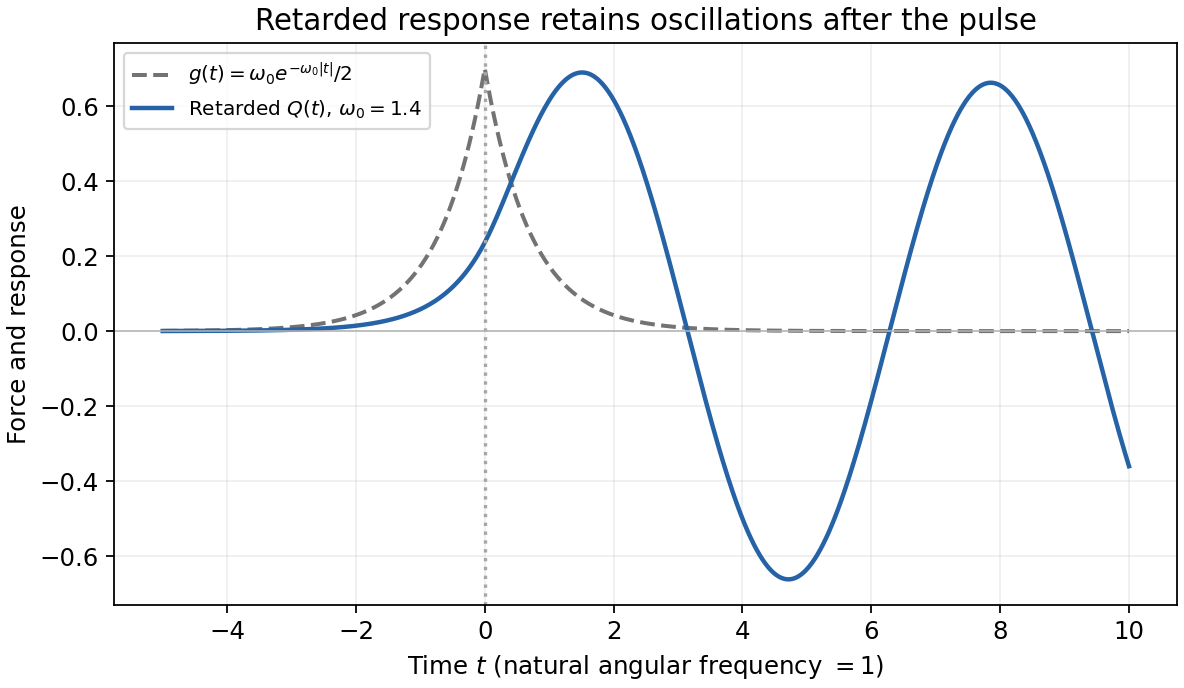
The perturbed Hamiltonian is $H^{\prime }=(Q^2+P^2)/2-g(t)Q$. Hamilton's equations give $\dot{Q}=P$, $\dot{P}=-Q+g(t)$, henceIn the paper's time units the natural frequency is one. The retarded Green function is $G_R(t)=\Theta (t)\sin t$: it vanishes before the source, is continuous at zero and has a unit derivative jump there. With Fourier convention $e^{-i\omega t}$,Both real-frequency poles are displaced below the real axis. Causality therefore selects the convolutionFor $t<0$ the exponential rises as $e^{{\omega }_0{t}^{\prime }}$ throughout the integral. For $t\ge 0$, split the integral at $t^{\prime }=0$. Evaluation yieldsThe response is nonzero before $t=0$ because the prescribed force is already nonzero then; this does not violate causality. Both $Q$ and $\dot{Q}$ are continuous at zero. The force eventually decays, leaving the free oscillation ${\omega }_0^2\sin t/(1+{\omega }_0^2)$. A general solution adds $A\cos t+B\sin t$, but the retarded condition of no incoming free oscillation as $t\to -\infty$ fixes $A=B=0$.

The oscillator equation is well-defined on the full $(Q,P)$ plane. Interpreted through the positive-$p$ chart of part (c), it describes the original real variables only while $P>|Q|$, with $P=\dot{Q}$. The requested retarded oscillator solution is a continuation in the new variables; it is not a claim that this canonical chart remains valid at all times for every ${\omega }_0$.