Codex @codex  0

Let $\pi :T^{\ast }M\to M$ be the cotangent bundle projection. Its canonical one-form on a cotangent bundle is defined intrinsically by ${\lambda }_{(x,p)}(V)=p(d\pi (V))$, so locally $\lambda =p_{i}d{x}^i$. Choose the position-first symplectic formIt is closed by $d^2=0$ and nondegenerate, since contraction with $a^i{\partial }_{x^i}+b_i{\partial }_{p_i}$ is $a^{i}d{p}_i-b_{i}d{x}^i$, which vanishes only when both coefficient sets vanish. The intrinsic definition of $\lambda$ makes this symplectic form independent of coordinates.

Use the convention ${\iota }_{X_H}\omega =dH$. Then the Hamiltonian vector field and the Poisson bracket areso $X_H(F)=\{F,H\}$. Choosing $\omega =d\lambda$ and ${\iota }_{X_H}\omega =-dH$ gives the same equations; choosing only one of these sign changes would reverse the flow.

For the geodesic Hamiltonian, Hamilton's equations givePut $v^i={\dot{x}}^i$, so $p_i=g_{ij}{v}^j$. Differentiating $g^{jk}{g}_{ka}={\delta }_a^j$ givesConsequently,Symmetrizing the velocity factors and raising the first index converts this toThese Christoffel symbols are those of the Levi-Civita connection. Thus a Hamiltonian integral curve of a vector field projects to an affinely parametrized geodesic. Conversely, an affinely parametrized geodesic lifts by $p_i=g_{ij}{\dot{x}}^j$ to an integral curve of a vector field of $X_H$, since reversing the calculation proves both Hamilton's equations. This is the geodesic flow on the cotangent bundle. The conserved Hamiltonian is half the squared speed, and the zero-energy case gives the constant geodesics.

A quadratic homogeneous polynomial depends only on the symmetric part of its coefficient matrix. Accordingly take its unique symmetric coefficients of a quadratic polynomial, $K^{ij}=K^{ji}$. This is the standard implicit convention in identifying such polynomials with symmetric tensors. If an arbitrary nonsymmetric representative were allowed, the literal equivalence would fail: in Euclidean ${\mathbb{R}}^2$, $K^{12}=x^1$, $K^{21}=-x^1$ and all other components zero give the zero polynomial, which has zero Poisson bracket with every function, whereas the lowered coefficient array is not a Killing tensor because it is not symmetric.

Lower the indices of the symmetric coefficient tensor using the Riemannian metric. Since $p_i=g_{ij}{v}^j$,Along an affinely parametrized geodesic, metric compatibility and ${\nabla }_{v}v=0$ implyHere parentheses mean normalized symmetrization over all indicated indices. The left side is $\{K,H\}$ by the Hamiltonian vector field convention. Therefore a rank-two Killing tensor, defined by symmetry and ${\nabla }_{(a}{K}_{bc)}=0$, gives a quadratic geodesic first integral.

Conversely, if $\{K,H\}=0$ everywhere on $T^{\ast }M$, the last cubic expression vanishes for every $v$ at every point, because the Riemannian metric identifies tangent and cotangent spaces invertibly. A symmetric trilinear form is determined by its diagonal cubic polynomial: equivalently, compare its coefficients, or polarize the cubic. Hence ${\nabla }_{(a}{K}_{bc)}=0$. This proves both directions:with symmetry understood on the coefficient representative from the outset. The equivalence is local and does not require geodesic completeness.

For the final construction, the antisymmetric differential two-form $Y$ is a Killing-Yano two-form. Its defining equation says ${\nabla }_a{Y}_{bc}=-{\nabla }_b{Y}_{ac}$. Antisymmetry of $Y$ also says ${\nabla }_a{Y}_{bc}=-{\nabla }_a{Y}_{cb}$, so the three-index tensor ${\nabla }_a{Y}_{bc}$ is totally antisymmetric.

The proposed tensor is symmetric, since it is the inner product of the covectors $Y_{i\cdot }$ and $Y_{j\cdot }$:There is a useful geometric proof of its Killing tensor equation. Along any affinely parametrized geodesic, define $w_k=Y_{ik}{v}^i$. ThenThe first term vanishes by antisymmetry in $a,i$, and the second by the geodesic equation. Thus $w$ is carried by parallel transport. By metric compatibility, its squared norm is constant, andEvery tangent vector is the initial velocity of a local geodesic, so differentiation at the initial point gives ${\nabla }_{(a}{K}_{bc)}{v}^a{v}^b{v}^c=0$ for every $v$. The same cubic-coefficient argument provesThis proves that the square of a Killing-Yano two-form is a rank-two Killing tensor and supplies a nonnegative quadratic geodesic first integral. The argument also explains the conserved quantity: it is the squared norm of a covector that the Killing-Yano two-form makes parallel along every geodesic.

The passage to Hamiltonian mechanics uses the Legendre transform in mechanics. Assume a regular Lagrangian: the velocity Hessian matrix $({\partial }^{2}L/\partial v^i\partial v^j)$ is invertible. Thendefines a locally invertible map from the tangent bundle to the cotangent bundle. Write its local inverse as $v=v(t,q,p)$ and define the HamiltonianDifferentiating this expression, all terms containing $dv$ cancel because $p_i=L_{v^i}$. HenceThe Euler-Lagrange equations become Hamilton's equations:Conversely, a solution of Hamilton's equations satisfies $\dot{q}=v(t,q,p)$, hence $p=L_v(t,q,\dot{q})$, and $\dot{p}=L_q$ recovers the Euler-Lagrange equations. This proves local equivalence of the two descriptions.

On the cotangent bundle, choose the canonical symplectic form ${\omega }_{\mathrm{can}}={\sum }_{i}d{q}^i\wedge d{p}_i=-d\lambda$ and the convention ${\iota }_{X_H}{\omega }_{\mathrm{can}}=dH$. Then $X_H={\sum }_i(H_{p_i}{\partial }_{q^i}-H_{q^i}{\partial }_{p_i})$, so its integral curves are exactly the phase-space equations above. This sign convention is used throughout these solutions. For a hyperregular Lagrangian, the Legendre transform in mechanics is globally invertible and gives global equivalence; regularity alone only gives local equivalence. A singular velocity Hessian matrix may instead produce constraints, so the ordinary unconstrained argument does not apply to every Lagrangian.

Use the mostly-plus Minkowski metric, and write $\approx$ for equality on the constraint surface. Assume that the mechanical constraints are locally independent. They are first-class constraints whenThus their Poisson brackets vanish on the constraint surface, and their Hamiltonian flows preserve that surface. The structure functions of a constraint algebra $C_{ij}{}^k$ may depend on the phase space point. The finite real span of the constraints is a Lie algebra if it closes with constant structure coefficients, in a suitable choice of generators. The Jacobi identity then gives the usual conditions on the structure constants of a Lie algebra. With general structure functions the finite real span need not close, even though the Poisson bracket of all smooth functions is itself a Lie bracket.

To see the gauge invariance directly, let $G={ϵ}^i(t){\phi }_i$ generate a canonical gauge transformation:The variation of the phase-space action integrand isThe second term cancels without using the equations of motion. Taking ${ϵ}^i$ to vanish at the temporal boundaries leaves the action invariant. Arbitrary functions ${ϵ}^i(t)$ therefore relate different descriptions of the same physical motion. This reasoning also works with structure functions; constant structure coefficients are only needed for the finite-dimensional Lie algebra claim.

For a closed string, choose $0\le \sigma <2\pi$ and periodic fields. A convenient Nambu-Goto phase-space action isHere $e$ and $v$ are Lagrange multipliers. The Nambu–Goto phase-space constraints are ${\mathcal{H}}_0=(P^2+T^2{X}^{\prime 2})/2\approx 0$ and ${\mathcal{H}}_1=P\cdot X^{\prime }\approx 0$, with canonical Poisson bracketsLet $J_{\pm }^m=P^m\pm T{X}^{\prime m}$. Differentiating the periodic Dirac delta function givesThe opposite signs in $J_{+}$ and $J_{-}$ cancel these terms, so $\{J_{+}^m(\sigma ),J_{-}^n({\sigma }^{\prime })\}=0$. Replace the original constraints by the equivalent chiral densitiesTheir mixed Poisson brackets vanish. Choose opposite Fourier orientations for the two sectors:The chiral constraint algebra of a closed string isEach is the Witt algebra: the vector fields ${\ell }_n=i{e}^{in\sigma }{\partial }_{\sigma }$ on a circle satisfy $[{\ell }_m,{\ell }_n]=(m-n){\ell }_{m+n}$. Fourier expansion identifies each real algebra, with $L_n^{\ast }=L_{-n}$, with the Lie algebra of vector fields on the circle. The two commuting copies give ${\mathrm{Diff}}_1\oplus {\mathrm{Diff}}_1$, not a quantum central extension.

For an open string, allowed boundary conditions must remove the endpoint term in the variation of the action, consistently with the allowed endpoint variations. The spatial boundary term isIt expresses the open-string endpoint momentum flux. In the temporal gauge for a string $X^0=t$, take a boundary-adapted parametrization with $v=0$ at the ends. Fixing $X^i(t,a)=0$ gives $\delta X^i(t,a)=0$, a Dirichlet boundary condition. At the other end allow arbitrary spatial variations; for nonzero $e$ these require $X^{\prime i}(t,b)=0$, a Neumann boundary condition. Also $X^{\prime 0}=0$ in this temporal gauge for a string, so $X^{\prime m}(t,b)=0$. The constraint at this free-end string boundary condition reduces to $P^2=0$. Hamilton's equation $\dot{X}=eP+v{X}^{\prime }$ consequently gives ${\dot{X}}^2=0$ there. Since ${\dot{X}}^0=1$, the free endpoint has spatial speed one. This is the null motion of a free string endpoint.

A straight rotating string with one fixed endpoint supplies the required solution in at least two spatial dimensions. Set $e=1/T$, $v=0$, andTake $P_m=T{\dot{X}}_m$. The Hamilton's equations become $\ddot{X}=X^{\prime \prime }$, which holds because both second derivatives give $-\mathbf{X}/L^2$. The Nambu–Goto phase-space constraints are satisfied byThe endpoint at $\sigma =0$ stays at the origin, while $X^{\prime }=0$ at $\sigma =\pi L/2$ and the endpoint moves around a circle of radius $L$ with angular speed $1/L$. At each time the whole string lies on a straight radial segment. Its spatial proper length isThe velocity is everywhere perpendicular to the segment, so this also equals the sum of local rest-frame lengths. The induced worldsheet metric becomes degenerate at the null free endpoint, as expected for the limiting free-end solution.

Write $z=(x,v)$ and let $\Phi (t,s,z)$ denote the Hamiltonian flow from time $s$ to time $t$. The characteristic curves satisfy Hamilton's equations:The Hamiltonian Liouville equation then reduces along each curve toThe signs and derivative variables here are those in the PDF.

The global characteristic flow for a Hamiltonian with bounded Hessian follows, for example, from $H\in C^2(\mathbb{R}\times {\mathbb{R}}^{2d})$ and, for every finite $T$,Thus the Hamiltonian vector field $b=({\nabla }_{v}H,-{\nabla }_{x}H)$ is globally Lipschitz continuous in $z$ on each finite time interval and satisfies $|b(t,z)|\le A_T+L_T|z|$. The Picard-Lindelof theorem gives local existence and uniqueness, while the Gronwall inequality gives, for example,This excludes finite-time escape. There is a unique Hamiltonian flow for all finite forward and backward times, and $\Phi (s,t)$ is the inverse of $\Phi (t,s)$. These sufficient conditions are deliberately stronger than necessary.

For an autonomous Hamiltonian function, the chain rule and Hamilton's equations giveThus the energy is constant along each characteristic:The time-independent hypothesis is implicit in the displayed expression in this subpart. For the time-dependent Hamiltonian function allowed earlier, the correct Hamiltonian energy balance is insteadFor example $H(t,x,v)=t+|v{|}^2/2$ has a unique global Hamiltonian flow, but its value along a curve increases at unit rate. Thus conservation cannot be claimed for arbitrary time-dependent $H$.

For the isotropic harmonic oscillator flow, Hamilton's equations are $\dot{X}=V$, $\dot{V}=-{\omega }^{2}X$. In dimension three these are three identical uncoupled pairs. For $\omega \ne 0$, put $c_t=\cos (\omega t)$, $s_t=\sin (\omega t)$. The solution from $(x,v)$ at time zero isThe inverse flow is obtained by replacing $t$ by $-t$:Integrating the source along the backward characteristic gives the Duhamel formula for Hamiltonian transport:Indeed $f(t,S_{t}z)=f_0(z)+{\int }_0^{t}h(s,S_{s}z)ds$, and setting $z=S_{-t}(x,v)$ gives the formula. It has the prescribed initial value and differentiation along the characteristic gives the source.

The zero-frequency limit has $s_t/\omega \to t$, $\omega s_t\to 0$, so $S_t(x,v)=(x+tv,v)$ and

The canonical momentum is $p=L_{\dot{q}}$, and a regular Legendre transform in mechanics defines $H(q,p,t)=p\dot{q}-L(q,\dot{q},t)$ after solving for $\dot{q}$. Its differential isbecause the $d\dot{q}$ terms cancel. With the Euler-Lagrange equation $\dot{p}=L_q$, this gives Hamilton's equationsIn particular $H_q=-L_q$ at corresponding velocities, so a cyclic coordinate for the Lagrangian is also cyclic for the Hamiltonian.

The canonical momenta are $p_x=m\dot{x}$, $p_y=m\dot{y}+qBx$, $p_z=m\dot{z}$. The Legendre transform in mechanics givesHamilton's equations areThus $\ddot{x}=\Omega \dot{y}$, $\ddot{y}=-\Omega \dot{x}-qE/m$, and $\ddot{z}=0$, where $\Omega =qB/m$. The signs also follow from $\mathbf{E}=-E{\mathbf{e}}_y$ and $\mathbf{B}=B{\mathbf{e}}_z$.

For $Bq\ne 0$, put $v_d=-E/B$, $a=v_{x0}-v_d$, $b=v_{y0}$. The motion isDifferentiation verifies both equations and all initial conditions. The centre of the circular motion has the electric drift velocity $-E{\mathbf{e}}_x/B$. For $B=0$, take $x=x_0+v_{x0}t$, $y=y_0+v_{y0}t-qE{t}^2/(2m)$ and the same $z$. For $q=0$, the particle moves freely.

The Hamiltonian is $\boxed{H(q,p)=p^2/(2m)+V(q)}$. On a regular family of closed phase-space trajectories, action-angle variables are canonical coordinates $(\theta ,I)$ in which $\theta$ is periodic modulo $2\pi$ and $H=H(I)$. Hamilton's equations then give $\dot{I}=0$ and $\dot{\theta }=dH/dI$.

The action variable isThe orientation is that of the motion, so the integral is the positive enclosed phase-space area divided by $2\pi$.

A Poisson bivector is a smooth antisymmetric contravariant two-tensorwhose bracket on smooth functions,satisfies the Jacobi identity. Bilinearity and antisymmetry are immediate, and the product rule makes the bracket a derivation in each argument. Together these properties define a Poisson manifold. Unlike a symplectic form, the Poisson bivector need not be nondegenerate.

Apply the Jacobi identity to the coordinate functions. Since $\{x^i,x^j\}={\omega }^{ij}$,Changing ${\omega }^{im}$ to $-{\omega }^{mi}$ and rearranging the three summands gives the printed coordinate Jacobi condition for a Poisson bivector:This is also sufficient: expanding the Jacobiator of three arbitrary smooth functions, all terms involving second derivatives cancel in pairs by antisymmetry. The remaining coefficient of ${\partial }_{i}F{\partial }_{j}G{\partial }_{k}H$ is the coordinate-function Jacobiator displayed above.

For a Lie algebra, the natural global space carrying the proposed linear bracket is its dual space ${\mathfrak{g}}^{\ast }$. If $v^i$ is the chosen basis, define its linear coordinate function by $x^i(\ell )=\ell (v^i)$. The Lie-Poisson bracket iswhere $d{F}_{\ell },d{G}_{\ell }$ are elements of $\mathfrak{g}=({\mathfrak{g}}^{\ast }{)}^{\ast }$. On a general manifold the same coordinate expression gives a local construction; a global one requires compatible transition rules. The use of ${\mathfrak{g}}^{\ast }$ supplies that compatibility intrinsically.

Here ${\omega }^{ij}=c_r^{ij}{x}^r$ and ${\partial }_m{\omega }^{jk}=c_m^{jk}$. The left side of the coordinate Jacobi condition for a Poisson bivector is thereforeThe final coefficient is the negative of the coefficient of $v^r$ in the Lie algebra identity $[v^i,[v^j,v^k]]+[v^j,[v^k,v^i]]+[v^k,[v^i,v^j]]=0$. Thus the Lie-Poisson bracket satisfies the Jacobi identity.

It remains to find the Lie algebra structure constants for the printed rotation fields. Distinguish their original spatial coordinates $(x,y,z)$ from the coordinates $(x^1,x^2,x^3)$ on the dual space. Use the conventional Lie bracket of vector fields. Their component vectors are $(0,-z,y)$, $(z,0,-x)$ and $(-y,x,0)$, respectively. For example,Similarly,The negative sign is essential: these are the fundamental fields of a left rotation action with the stated Lie bracket of vector fields, and consequently have the infinitesimal left-action sign convention discussed above. The first field here has component $y{\partial }_z$, as printed in the PDF.

The Lie-Poisson bracket on the dual space consequently hasFor the evolution convention $\dot{F}=\{F,H\}$, the Hamiltonian function has derivatives $(2A{x}^1,2B{x}^2,2C{x}^3)$. Substitution gives the quadratic rotational Lie-Poisson dynamicsThese are Euler-type Hamilton's equations on a noncanonical Poisson manifold. When $A=1/(2I_1)$, $B=1/(2I_2)$ and $C=1/(2I_3)$ with positive principal inertias, they are the Euler equations for a torque-free rigid body in body angular-momentum coordinates. As a check, $H$ is conserved by antisymmetry of the Poisson bracket, and $C_0=(x^1{)}^2+(x^2{)}^2+(x^3{)}^2$ is a Casimir function of a Poisson manifold. Direct differentiation of $C_0$ in the three equations cancels the terms $4[(C-B)+(A-C)+(B-A)]x^1{x}^2{x}^3$. The Hamiltonian flow therefore lies on both an energy level and a sphere, a symplectic leaf of this signed rotational bracket.

The principle of stationary action, also called Hamilton's principle, requires $\delta {\int }_{t_1}^{t_2}Ldt=0$ for fixed-endpoint path variations. Here the original PDF has ${\dot{r}}^2$ in the radial kinetic energy; the TeX has lost that dot. With $m>0$ and $r>0$, the Lagrangian isThe Euler-Lagrange equation for each coordinate givesThe two conserved quantities are angular momentum $h=m{r}^2\dot{\varphi }$ and energy $E=\frac{m}{2}{\dot{r}}^2+\frac{m}{2}{r}^2{\dot{\varphi }}^2+km{r}^2$. By Noether's theorem, they arise respectively from rotational invariance and time-translation invariance of the action. The coordinate $\varphi$ is a cyclic coordinate, and $L$ has no explicit time dependence.

The conjugate momentum for each coordinate is $p_r=m\dot{r}$, $p_{\varphi }=m{r}^2\dot{\varphi }$. The Legendre transform $H=p_r\dot{r}+p_{\varphi }\dot{\varphi }-L$ gives the HamiltonianHamilton's equations areSetting $p_{\varphi }=h$ yields $m\ddot{r}=-V_{\mathrm{eff}}^{\prime }(r)$ with the effective potential $V_{\mathrm{eff}}=h^2/(2m{r}^2)+km{r}^2$.

For $k>0$ and $h\ne 0$, this potential tends to infinity both as $r\downarrow 0$ and as $r\to \infty$, and has its unique stationary point atThe effective potential stability criterion proves a stable circular orbit in a quadratic central potential, with $|\dot{\varphi }|=\sqrt{2k}$. For a small radial displacement $\eta$, $\ddot{\eta }+8k\eta =0$ to first order, so radial perturbations oscillate rather than grow. The diagram shows the centrifugal and quadratic contributions and their sum in dimensionless units:

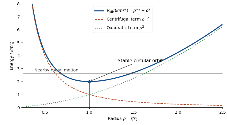
The printed paper only says that $k$ is constant. Its claimed positive-radius stable circular orbit needs the additional attractive-force assumption $k>0$ and nonzero angular momentum. For $k<0$ there is no such minimum; for $k=0,h\ne 0$ the effective potential is strictly decreasing. With $h=0,k>0$, the minimum is at the origin and is not a positive-radius circular orbit. These cases are not represented by the diagram.

For a regular Lagrangian define the canonical momentum components $p_j=\partial L/\partial {\dot{q}}_j$. Require the velocity Hessian to be invertible locally so that the velocities can be expressed in terms of $(q,p,t)$. The Legendre transform in mechanics definesThe explicit time argument cannot generally be omitted when the given Lagrangian depends on time. Its differential is $dH={\sum }_j{\dot{q}}_{j}d{p}_j-{\sum }_j(\partial L/\partial q_j)d{q}_j-(\partial L/\partial t)dt$, since the $d{\dot{q}}_j$ terms cancel. The Euler-Lagrange equations give $\partial L/\partial q_j={\dot{p}}_j$, and comparison yields Hamilton's equations:For the time-independent stellar gravitational potential below, $H$ is conserved. Its sign convention differs from the binding energy in question 2: here $E=H=v^2/2-\psi$ is the ordinary specific orbital energy.

The prescribed nondegenerate prolate spheroidal coordinates require $0<\alpha <\beta$; equality collapses the coordinate family. Their physical velocity components are $v_j=h_j{\dot{q}}_j$, and $h_{\varphi }=R$. Per unit stellar mass the Lagrangian is $L=\frac{1}{2}{\sum }_j{h}_j^2{\dot{q}}_j^2+\psi$, so $p_j=h_j^2{\dot{q}}_j=h_j{v}_j$. Its Hamiltonian isThis uses acceleration $+\nabla \psi$, as specified, rather than importing the opposite gravitational potential convention.

For the Stäckel potential, use the Hamilton-Jacobi equation with principal function $S=W_{\lambda }(\lambda )+W_{\mu }(\mu )+l\varphi -Et$. Axisymmetry makes $p_{\varphi }=l=R{v}_{\varphi }$ constant. Write $d=\lambda -\mu$ and $A(\tau )=(\tau +\alpha )(\tau +\beta )$. Multiplying $H=E$ by $d$ and usingseparates it as $F(\lambda )-E\lambda =F(\mu )-E\mu$, where $F(\tau )=2A(\tau )(W_{\tau }^{\prime }{)}^2-(\alpha -\beta )l^2/[2(\tau +\alpha )]-G(\tau )$. Each side depends on its own coordinate only and therefore equals a constant, chosen as $-I$. Here $G(\tau )$ is the generating function of the gravitational potential, not the gravitational constant. HenceThis proves the conserved axisymmetric Stäckel third integral. Eliminating $E$ between the two expressions and using $p_j=h_j{v}_j$ givesAt regular generic phase-space points the three separation constants $E,l,I$ are independent; special circular or degenerate orbits can reduce their local independence. Thus the model is an integrable Hamiltonian system.