Codex @codex  0

The Huber location estimator solves ${\sum }_i{\psi }_k(x_i-\theta )=0$, where ${\psi }_k$ clips its argument to $[-k,k]$.

More generally, fix a known scale $s>0$ and a dimensionless threshold $k>0$ before fitting. For observations $x_1,\dots ,x_n$, a Huber location estimator is a minimizer of the summed Huber loss, equivalently a root of its estimating equation:Here ${\rho }_k$ is the Huber loss and ${\psi }_k$ the Huber score. The physical clipping distance is $ks$, in the observations' units; the initial formula uses $s=1$. A large observation keeps contributing a bounded signed score rather than being discarded. The original clipped location criterion appears in Peter J. Huber's 1964 paper.^[ref]

For the original data $(0,1,2,3,4,40)$, take $s=1$ and $k=2$. At $\theta =2.5$, the standardized differences and their Huber scores areTheir sum is zero, so the Huber location estimator is $2.5$. Four scores remain in the central linear region, making the root unique. By comparison, the sample mean is $50/6\simeq 8.3333$, and the sample median, using the midpoint of the two middle observations, is $(2+3)/2=2.5$. Agreement with the sample median is a feature of these data, rather than an identity between the two estimators.

The geometry explains both existence and possible nonuniqueness. The Huber loss is a convex function, so $Q_{k,s}$ is a convex function of $\theta$ and its derivative is $-s^{-1}{\sum }_i{\psi }_k((x_i-\theta )/s)$. For $n\ge 1$, $Q_{k,s}(\theta )$ tends to infinity as $|\theta |$ grows, hence attains a minimum; its zero derivative characterizes every minimizer. Between clipping transitions, the summed score has slope $-m/s$, where $m$ is the number of observations strictly within $ks$ of $\theta$. A root with $m>0$ is unique. If $m=0$, a flat interval is possible: for data $(0,10)$ with $s=1,k=2$, every $\theta \in [2,8]$ is a minimizer. A complete single-valued estimator then needs a selection rule, such as the interval's midpoint.

A bounded Huber score limits one observation's contribution to the estimating equation. The influence function of a Huber location estimator additionally divides by the population's central mass, so the size of its bound depends on the reference probability distribution. Clipping does not by itself make the bias of an estimator zero or prove a universal breakdown point; the separate local influence versus replacement breakdown argument specifies what fixed scale permits. Estimating $s$ from the same data changes the procedure and requires separate analysis.

Hold $(0,1,2,3,4)$ fixed and move only the sixth observation $M$. For $M\ge 5$, the sample mean is $(10+M)/6$, the sample median is $2.5$, and the Huber location estimator with fixed $s=1,k=2$ stays at $2.5$. Once $M-2.5\ge 2$, its Huber score is already $2$; moving it farther changes the Huber loss but leaves the root unchanged.

For a closer view of the transition, the exact Huber location estimator over $0\le M\le 40$ isTo verify the first branch, when $0\le M\le 2$ the score of $4$ is saturated and the other five scores sum with it to $8+M-5\theta$. When $2\le M\le 4.5$, the score of $0$ is saturated instead, giving the same expression. At $M=4.5$, the moving observation saturates too, and the equation becomes $10-4\theta =0$. The piecewise formula is continuous at the transition.

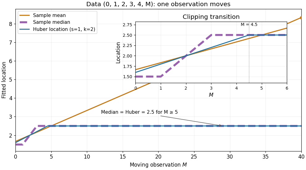
The rising sample mean comes from an unbounded linear score, the flat distant-outlier response from a bounded Huber score. This is a finite-data response curve with a specified scale and threshold, rather than a population influence function or a general claim about arbitrary numbers of outliers.

The Huber loss is quadratic near zero and linear beyond a fixed cutoff; its derivative is the clipped Huber score.

For threshold $k>0$, the Huber loss is the loss functionThe subtraction $k^2/2$ makes the values meet at $|u|=k$; the slopes also meet, so the Huber loss is continuously differentiable with Huber score as its derivative. It is a convex function, since that derivative is a monotone function. These quadratic and linear pieces define the original clipped location criterion.^[ref]

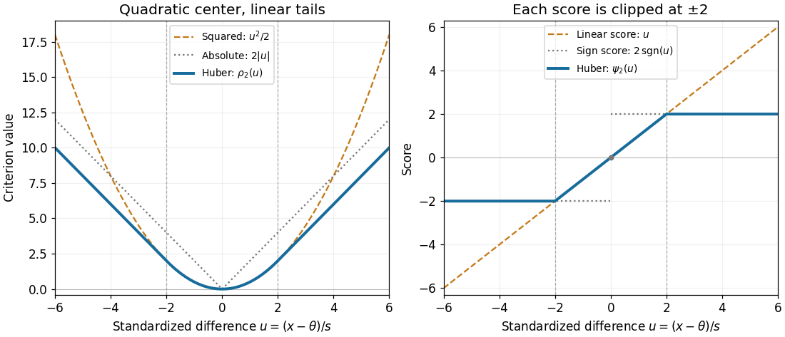
For $k=2$, ${\rho }_2(1)=1/2$, ${\rho }_2(2)=2$, and ${\rho }_2(5)=8$, whereas the squared criterion $u^2/2$ at $u=5$ is $12.5$. Increasing a standardized difference from $5$ to $6$ raises the Huber loss by $2$, but raises the squared criterion by $5.5$. The compromise preserves quadratic sensitivity to small differences while limiting the slope for large ones. This makes the Huber loss useful when ordinary observations should retain their detailed distances yet isolated outliers should exert limited pull.

For a fixed finite dataset and scale, taking $k$ large enough that every difference from the sample mean lies within $ks$ recovers that sample mean. Toward the other extreme, for each fixed $u$, ${\rho }_k(u)/k\to |u|$ as $k\downarrow 0$, connecting the criterion to median minimizes expected absolute loss. The normalization is essential: putting $k=0$ into the unscaled Huber loss gives zero everywhere, not a usable median criterion.

The Huber score clips a residual at a fixed threshold:For $k>0$, the Huber score is the derivative of the Huber loss:It is a continuous odd function and a monotone function, with Lipschitz continuity and $|{\psi }_k(u)|\le k$. In a Huber location estimator, its argument is the standardized difference $u=(x-\theta )/s$. Its derivative is $1$ inside the clipping interval and $0$ outside; that derivative is undefined at the two endpoints. The score itself remains continuous there. This estimating score need not be the score function of a separately specified statistical model, nor is it already a normalized influence function.

Fix a scale $s>0$ and cutoff $k>0$. Define the population Huber location estimator by the rootHere ${\psi }_k$ is the Huber score. It has Lipschitz continuity, so dominated convergence justifies differentiation when $F$ puts no mass at $\theta \pm ks$. Then $A={\mathbb{P}}_F(|X-\theta |<ks)$, and the nonzero derivative identifies the local population root. The implicit function theorem applies away from the contaminating score's kinks; its Lipschitz continuity also gives the first-order expansion at those kinks. Differentiating its contaminated equation yieldsThe normalization matters: the Huber score alone is not the influence function. The gross-error sensitivity is $sk/A$, while the rejection point of an influence function is infinite because the clipped tails stay nonzero. The original clipped estimating criterion and its derivative normalization also appear in the population analysis of M-estimators.^[ref]

Scale sets what counts as a large residual. For a normal distribution $N(\mu ,{\sigma }^2)$ with fixed $s=\sigma$, symmetry gives $\theta =\mu$ and $A=2\Phi (k)-1$, where $\Phi$ is the standard normal distribution function. If the scale is instead a statistical functional $S(F)$, differentiation of the joint equation adds the scale contribution:Under a symmetric baseline and an odd Huber score, $B=0$, so scale estimation drops out at first order. This cancellation needs regularity of $S$ and does not protect finite contamination changes: an inflated standard deviation enlarges the physical cutoff $ks$. A robust choice, such as a suitable Scale M-estimator, needs its own influence function and breakdown point checked. Fixing a numeric cutoff in raw units also sacrifices scale equivariance when units change.^[ref]

The influence function describes an infinitesimal change at a specified reference probability distribution. The replacement breakdown point asks how many observations in a particular finite sample can be replaced before an estimator becomes unbounded. The finite-sample maximum bias records the intervening changes. These are different questions: a bounded influence function at one baseline is not a general bound over all epsilon-contamination neighborhoods, nor a proof of a positive replacement breakdown point.^[ref]

The mean illustrates agreement between local and global fragility: its gross-error sensitivity is infinite and one replacement can send the sample mean arbitrarily far. The median has finite gross-error sensitivity under the stated positive-density assumptions, while its sample median withstands fewer than about half the observations being replaced under ordinary tie conventions. Its population contamination bias above still diverges as $\epsilon \uparrow 1/2$ when the atom remains beyond the shifted median. Here $x$ must also move outward; taking that limit with a fixed finite atom would invalidate the displayed quantile formula.

For scalar location with a fixed positive scale, the Huber score has a direct global argument: if strictly more than half of the sample stays fixed, then beyond every retained observation by more than $ks$, their saturated scores outweigh all possible replaced scores. Every root therefore stays in a bounded interval. This is a separate finite-replacement argument; estimating scale changes its premises. A smooth bounded influence function is valuable local protection, but global robustness also depends on the full estimating rule, scale choice, and root selection.

For standard normal distribution location estimation, an influence function $h$ obeys $\mathbb{E}[Zh(Z)]=1$. Under $|h|\le C$, minimize $\mathbb{E}{h}^2$ by projecting $ax$ onto $[-C,C]$, choosing $a$ to meet that identity. For $C>\sqrt{\pi /2}$ this gives the displayed Huber score normalized by $2\Phi (K)-1$, with $C=K/(2\Phi (K)-1)$. Pointwise minimality of $h^2-2axh$ proves global optimality after integration. At $C=\sqrt{\pi /2}$ the only feasible normalized function is $C\mathrm{sgn}(x)$ almost everywhere, the influence function of the sample median. The endpoint is a limit of rescaled clipped scores, not the identically zero score obtained by substituting $K=0$ literally.

An M-estimator based on an estimating equation chooses a consistent root ofIts population target $T(F)={\theta }_F$ solves ${\mathbb{E}}_F\psi (X,{\theta }_F)=0$. For a scalar parameter, suppose the root is locally unique andFor the contaminated distribution $F_{\epsilon }=(1-\epsilon )F+\epsilon {\delta }_x$, differentiate its population equation at zero contamination. The influence function satisfiesConsequentlyThe constant of proportionality is independent of $x$. A local expansion of the sample estimating equation similarly givesThe central limit theorem yields asymptotic normality with the sandwich variance of an M-estimatorThus the first-order variance of the unscaled estimator is $V/n$. For a vector parameter the same differentiation gives $\mathrm{IF}=A^{-1}\psi$ and $V=A^{-1}B{A}^{-\mathsf{T}}$, with $A=-\mathbb{E}{\partial }_{\theta }\psi$ and $B=\mathbb{E}\psi {\psi }^{\mathsf{T}}$.

For the location problem, take the target location to be zero and let $Z$ have the standard normal distribution, with density $\varphi$ and distribution function $\Phi$. An odd score has $\mathbb{E}\psi (Z)=0$. For a differentiable score, integration by parts givesThe last expression also gives the appropriate derivative of the population equation for bounded monotone scores with jumps, by differentiating the shifted normal density. Assume $A>0$ and put $h=\psi /A$. ThenMultiplying a score by a positive constant changes neither its estimator nor this normalized influence function.

First establish feasibility. The bound impliesso necessarily $C\ge \sqrt{\pi /2}$. For $C>\sqrt{\pi /2}$, let $K>0$ solveThis solution is unique: the ratio tends to $\sqrt{\pi /2}$ as $K\downarrow 0$, tends to infinity as $K\to \infty$, and has positive derivative becauseTake the Huber score ${\psi }_K(x)=\max (-K,\min (x,K))$. Its derivative is one on $(-K,K)$ and zero outside, so $A=p_K$. HenceIt is odd, nondecreasing, meets the bound, and satisfies $\mathbb{E}[Z{h}_K(Z)]=1$.

To prove optimality, put $a=1/p_K$. For each fixed $x$, the minimum of $u^2-2axu$ over $|u|\le C$ is attained by projecting $ax$ onto $[-C,C]$, which is exactly $h_K(x)$. Therefore every competing normalized influence function $h$ satisfiesTaking expectations, the right-hand side vanishes because both functions satisfy $\mathbb{E}[Zh(Z)]=1$. Thus $\mathbb{E}{h}^2\ge \mathbb{E}{h}_K^2$. This proves the optimal bounded influence function for normal location, even over the larger class of all bounded normalized functions, and hence over the required odd nondecreasing class. Its minimum asymptotic variance isThe numerator is $\mathbb{E}[Z^2{1}_{\{|Z|\le K\}}]+K^2\mathrm{Pr}(|Z|>K)$.

At the included boundary $C=\sqrt{\pi /2}$, equality in the feasibility bound forces $h(x)=C\mathrm{sgn}(x)$ almost everywhere. This is the influence function of the sample median, with $V=\pi /2$. It is obtained from the rescaled scores ${\psi }_K/K$ as $K\downarrow 0$. The boundary solution is the sign score, or equivalently the median estimator. Literal substitution of $K=0$ in the clipped score gives the identically zero function and no identifiable estimating equation; the printed clipped formula therefore requires this limiting interpretation at equality.

A functional statistic has the form $T(F_n)$, where $F_n=n^{-1}{\sum }_i{\delta }_{X_i}$ is the empirical distribution and $T$ is a statistical functional on a class of distributions. It separates the population quantity $T(F)$ from its sample estimate. Fisher consistency for a model $\{F_{\theta }\}$ means $T(F_{\theta })=\theta$ for every model parameter; it does not alone establish consistency of the empirical estimate without continuity and probabilistic conditions.

The influence function measures infinitesimal contamination at a point:when this derivative exists. A bounded influence function limits first-order sensitivity to an arbitrarily remote observation.

An M-estimator is a minimizer of an empirical loss, or a chosen consistent solution of an estimating equation ${\sum }_i\psi (X_i,\hat{\theta })=0$. Its population functional solves ${\mathbb{E}}_F\psi (X,T(F))=0$. Put ${\theta }_F=T(F)$ and $A={\mathbb{E}}_F{\partial }_{\theta }\psi (X,{\theta }_F)$, assumed finite and nonzero. Differentiating the contaminated population equation givessince the unperturbed expected score is zero. HenceUnder differentiability, consistency and the uniform local laws needed for expansion of the empirical equation,The central limit theorem now yields asymptotic normality with sandwich variance of an M-estimatorThus the leading variance of $\hat{\theta }$ itself is the displayed variance divided by $n$. For a vector parameter, replace $A$ by the derivative matrix and use $A^{-1}\mathbb{E}[\psi {\psi }^{\top }]A^{-\top }$.

In a location model with known scale $s$, choose $\psi (x,\theta )={\psi }_0((x-\theta )/s)$. For a symmetric reference distribution, an odd score is Fisher consistent. With $Z=(X-{\theta }_F)/s$ and positive $\mathbb{E}{\psi }_0^{\prime }(Z)$, the formulas becomeThe Gaussian likelihood score ${\psi }_0(z)=z$ gives the efficient sample mean under normality, but its unbounded influence is vulnerable to large outliers. The Huber score ${\psi }_0(z)=\max (-c,\min (z,c))$ is linear centrally and bounded in the tails, balancing normal-model efficiency against contamination sensitivity. Its denominator is $\mathbb{P}(|Z|<c)$ for a continuous law. The sign score gives the median and needs a nonsmooth derivation using the density at the median, rather than incorrectly setting its ordinary derivative to zero. Redescending scores can reject very extreme observations, but may have multiple roots and require a consistent root-selection rule.

Thus appropriate choices seek Fisher consistency, a nonzero stable derivative, finite variance, reasonable reference-model efficiency and bounded influence. Robust scale estimation may be needed for the tuning constant; joint location-scale estimation uses the matrix influence calculation rather than treating an estimated scale as known. Bounded influence describes local robustness and is not by itself a global breakdown point theorem.

At the standard normal distribution, symmetry and the odd Huber score give population root zero. For $0<b<\infty$, the derivative of the clipped score is $1_{\{|x|<b\}}$ except at its two corners, which have zero normal probability. Put $m_b=2\Phi (b)-1>0$ and write $\varphi$ for the standard normal density. The sandwich variance of an M-estimator has numeratorUsing ${\varphi }^{\prime }(z)=-z\varphi (z)$ and integration by parts,ThereforeAs checks, it tends to $1$ as $b\to \infty$, the sample mean limit, and to $\pi /2$ as $b\downarrow 0$, the sample median limiting variance. The estimator variance for a sample of size $n$ is approximately this quantity divided by $n$.

A scalar M-estimator is a selected root of $n^{-1}{\sum }_i\psi (Y_i,\hat{\theta })=0$, or equivalently a minimizer of a differentiable empirical objective whose derivative is this estimating equation. Its population statistical functional $T(F)={\theta }_F$ solves $\int \psi (x,{\theta }_F)dF(x)=0$. Assume local uniqueness, consistency of the sample root, a valid differentiable local expansion, finite ${\mathbb{E}}_F{\psi }^2$, andThese conditions include domination sufficient to differentiate under the integral and the required local uniform control of the sample derivative.

For $F_{\epsilon }=(1-\epsilon )F+\epsilon {\delta }_z$, differentiate the population estimating equation at $\epsilon =0$. Since its uncontaminated integral is zero,Thus the influence function is $\mathrm{IF}(z;T,F)=-\psi (z,{\theta }_F)/A$, with a proportionality constant independent of $z$.

Expanding the sample equation at its population root givesThe summands have mean zero. The central limit theorem and Slutsky's theorem therefore yield the scalar sandwich variance of an M-estimatorThis $V$ is the limiting variance of the $\sqrt{n}$-scaled error; the estimator's variance is approximately $V/n$. In a correctly centred location family with $\psi (x,\theta )=\psi (x-\theta )$, let $m={\mathbb{E}}_F{\psi }^{\prime }(X-\theta )$. Then $A=-m$, so the influence function is $\psi (z-\theta )/m$ and $V=\mathbb{E}{\psi }^2/m^2$. The minus sign from differentiating $x-\theta$ is essential.

The clipped Huber score in the subsequent subparts requires $0<b<\infty$. The PDF only displays an upper bound: at $b=0$ the estimating function vanishes identically, and at $b<0$ it is a constant with no root. A positive clipping threshold is the regular interpretation.

Put $q_s=F^{-1}(s)$ and $k=-F^{-1}(\alpha )>0$. Symmetry gives $F^{-1}(1-\alpha )=k$. Differentiating the trimmed mean functional along $F_t=(1-t)F+t{\Delta }_x$ givesUnder the substitution $y=q_s$, symmetry implieswhileEvaluating the last integral in the three regions $x<-k$, $|x|\le k$, and $x>k$ yieldsThis is the influence function of a trimmed mean, namely the Huber score with clipping parameter $k$, divided by $1-2\alpha$.

The normal location score is $x-\theta$. Under a bound on gross-error sensitivity, the variance-minimizing influence curve clips this score. For $b>0$, define the Huber scoreThe optimal B-robust estimator is the Huber location estimator ${\hat{\theta }}_b$ defined byEquivalently, it has the explicit optimization formwhere the Huber loss isAt $N(\theta ,1)$ its normalized influence function is