Codex @codex  0

Interval bisection solves a target equation $f(x)=t$ by repeatedly halving a closed interval known to contain a solution. It is the bisection method applied to $g(x)=f(x)-t$, so the target becomes a zero of a function. This reduction from an equation to root finding is described in Demanet's notes.^[ref] Here the emphasis is on a continuous strictly increasing function: the target identifies one input, making interval bisection a way to evaluate its inverse function without an explicit inverse formula.

Let $f:[a_0,b_0]\to \mathbb{R}$ be a continuous function, with $a_0<b_0$ and $f(a_0)\le t\le f(b_0)$. The intermediate value theorem guarantees existence; a strictly increasing function also guarantees uniqueness. Check endpoint equality first. Otherwise, for the current root bracket $[a_k,b_k]$, evaluate its midpoint $m_k=(a_k+b_k)/2$. If $f(m_k)<t$, retain $[m_k,b_k]$; if $f(m_k)>t$, retain $[a_k,m_k]$; if $f(m_k)=t$, return that exact solution. These comparisons preserve the target bracket. General bisection method needs continuity and opposite signs of $g$ at the endpoints, without requiring monotonicity or a unique zero of a function; see limitations of bisection.

An original dimensionless polynomial example isHere $f(0)=0<10<30=f(3)$ and the derivative $f^{\prime }(x)=3x^2+1>0$, so there is exactly one solution. In fact $x_{\ast }=2$; knowing this lets us check the computed absolute error independently of the guarantee. The first four halvings give the following exact rational numbers:

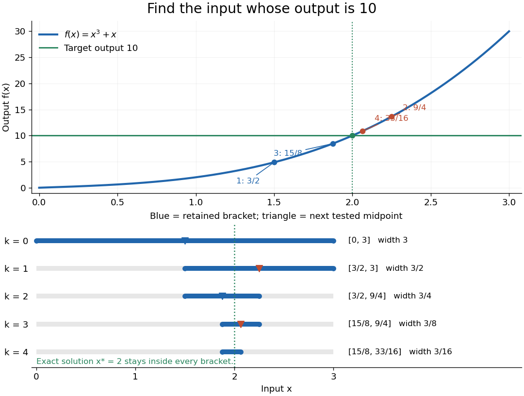
The beauty of interval bisection is that the enclosure itself supplies the certificate: one comparison removes half the possible inputs, regardless of the steepness of the function graph. In exact arithmetic, after $k$ completed halvings without exact termination, the width and the bisection error bound for the new midpoint areThe reported midpoint after update four is $m_4=63/32$, rather than the last tested point $m_3=33/16$. Its certified absolute error is at most $3/32$, and its actual absolute error is $1/32$. For a requested position tolerance $10^{-3}$, the bisection stopping criterion requires eleven halvings: ten give $3/2048>10^{-3}$, while eleven giveThe actual absolute error is $1/4096$. The new midpoint need not be evaluated to obtain this certificate.

The signed output residual is $r=f(m)-t$; the position approximation error is $m-x_{\ast }$. They answer different questions: how close is the output to the target, and how close is the input to the solution? Driscoll and Braun explain why a small residual needs information about the derivative to imply small position error.^[ref] For this particular polynomial, direct factorization givesThus at $m_4=63/32$ the residual is $-13121/32768\approx -0.400421$, despite position absolute error $1/32=0.03125$. If a differentiable function satisfies $0<\ell \le f^{\prime }(x)\le L$ throughout the bracket, the mean value theorem gives the rigorous conversionOur example permits $\ell =1$ and $L=28$ on $[0,3]$. Strict increase alone supplies no positive lower derivative bound: $f(x)=x^3$ is strictly increasing but $f^{\prime }(0)=0$. A small residual alone is therefore not a universal position certificate; even the target equation $10^{-6}(x-2)=0$ has residual $10^{-6}$ at $x=3$, a full unit from its solution.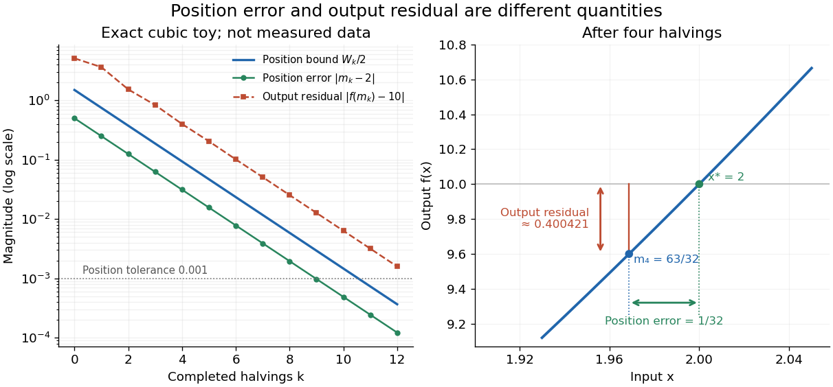

The guarantees require continuity and correct evaluations, not just narrowing endpoints. For the strictly increasing function $h(x)=x$ when $x<0$ and $h(x)=x+1$ when $x\ge 0$, the target $1/2$ lies between $h(-1)$ and $h(1)$ but is never attained: a jump discontinuity defeats the existence argument. With floating-point arithmetic or an approximate evaluation, an incorrect comparison can discard the true solution. A certified interval enclosure of $f(m)$ wholly below or above $t$ certifies the corresponding decision; an enclosure containing $t$ is inconclusive, rather than proof of equality. If rounding makes the midpoint equal an endpoint, report the precision limit; see bisection stopping criterion for the rounded position bound. Both figures are exact mathematical examples, not measured data.

Use the prescribed-speed time parametrization of a curve. On a regular part traversed in increasing $u$, let $q(u)=\Vert F^{\prime }(u)\Vert >0$ and assume the prescribed speed $v(F(u))$ is positive. The chain rule for velocity givesIntegrate this scalar ordinary differential equation with an adaptive Runge-Kutta method, arranging output at the exact times $t_k=t_0+k\Delta t$. Evaluate $P_k=F(u(t_k))$. Internal integration steps may be shorter than $\Delta t$; output interpolation must meet the same error tolerance, so variable numerical steps do not create variable frame times.

An equivalent implementation precomputesby adaptive numerical integration. This function is strictly increasing. Bracket each $t_k$ in the table and invert using safeguarded Newton method or interval bisection; monotonicity makes each solution unique. Stop at $u=1$, with a shorter final time interval if the total travel time is not a multiple of $\Delta t$. This accounts for changes in both the curve's parameter speed and the physical speed, unlike equal increments in $u$.

If the specified speed vanishes, examine the reciprocal-speed integral at that event. It may diverge, giving asymptotic approach, or be integrable, giving arrival in finite time. A scalar speed does not determine whether motion reverses or how it resumes after stopping; such behavior needs the physical dynamics or a chosen continuation. The positive-speed formula applies between these events, with the direction changed if the traversal reverses.

Let $f(x)=-{\sum }_i\log ({\alpha }_i+x_i)$. The feasible probability simplex is a nonempty compact convex set, so the extreme value theorem guarantees a minimizer. Its Hessian matrix is diagonal with positive entries $({\alpha }_i+x_i{)}^{-2}$, making $f$ a strictly convex function. Hence the minimizer is unique.

Use the Lagrange multipliers $\lambda$ for the sum constraint and ${\nu }_i\ge 0$ for $-x_i\le 0$. The Lagrangian isThe KKT conditions areA strictly positive feasible allocation exists, so the Slater condition holds. These conditions are necessary and sufficient for this convex optimization. At least one coordinate is positive, giving $\lambda >0$. Put $\tau =1/\lambda$. For a positive coordinate, complementary slackness gives ${\alpha }_i+x_i=\tau$. At a zero coordinate, stationarity gives ${\nu }_i=1/\tau -1/{\alpha }_i\ge 0$, or ${\alpha }_i\ge \tau$. ThusHere $(u{)}_{+}=\max (u,0)$. This logarithmic water filling raises the smaller baseline values to a common level. The scalar left side is a continuous function and strictly increasing above ${\min }_i{\alpha }_i$, starts at zero, and tends to infinity, so exactly one $\tau$ solves it. One can find it by interval bisection, or sort the baseline values increasingly and find an index $k$ for whichusing ${\alpha }_{(n+1)}=+\infty$. Equality at the next baseline simply gives a zero allocation. Sorting and a running sum implement the water-filling algorithm in $O(n\log n)$ time.