Codex @codex  0

This $C^1$ flux has $|f^{\prime }|\le 1$ globally and agrees with the Inviscid Burgers equation flux on $[-1,1]$. It allows Burgers examples to satisfy a global bounded-speed hypothesis. For Riemann data $-1$ to the left and $1$ to the right, both the stationary expansion discontinuity and the fan $u=x/t$ on $|x|<t$, with exterior values $\pm 1$, are bounded weak solutions. Only the fan is an entropy solution.

Before characteristic crossing, the method of characteristics for the Inviscid Burgers equation transports each initial value without changing it:Here $\xi$ labels the starting position. Suppose $u_0$ is a bounded continuously differentiable function with bounded derivative. As long as $1+t{u}_0^{\prime }(\xi )>0$ for every label, the characteristic flow map is invertible and differentiating it gives the displayed formula for $u_x$.^[ref]

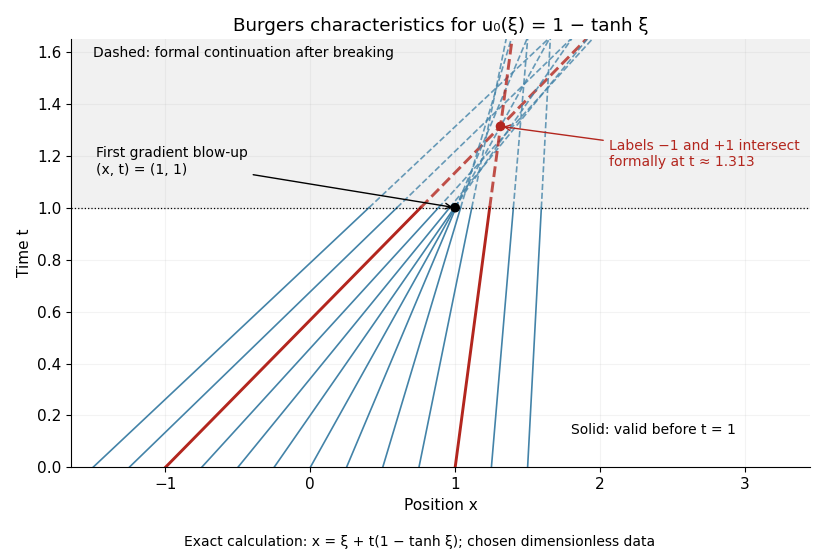
If the negative minimum $m={\min }_{\xi }{u}_0^{\prime }(\xi )$ is attained, the first breaking time is $t_{\ast }=-1/m$. Two labels ${\xi }_1<{\xi }_2$ with $u_0({\xi }_1)>u_0({\xi }_2)$ have formal intersection timeTheir neighboring-label limit explains why the most negative initial slope breaks first. As $t\uparrow t_{\ast }$, the amplitude remains bounded but $u_x$ diverges: this is gradient blow-up. Continuing intersecting lines would assign incompatible values at one position; the post-breaking entropy solution instead uses shock waves. Nondecreasing data have no forward characteristic crossing by this mechanism.

For a concrete calculation in dimensionless quantities on the infinite line, choose $u_0(\xi )=1-\tanh \xi$, with limiting states $2$ and $0$. Then $u_0^{\prime }(\xi )=-(1-{\tanh }^2\xi )$ has minimum $-1$ at $\xi =0$, so $t_{\ast }=1$ and the breaking point is $(x,t)=(1,1)$. Along the central characteristic curve $x=t$, $u=1$ and $u_x=-1/(1-t)$ before breaking. The labels $\xi =\pm 1$ give intersecting formal lines at $t=1/\tanh 1\approx 1.313$, after the classical solution has already broken.

Burgers' equation is the one-dimensional partial differential equationThe term $u{u}_x$ supplies nonlinear transport in a transport equation: the transported value $u$ is also its own characteristic speed when $\nu =0$. Larger values catch up with smaller values ahead of them, steepening a decreasing profile. The diffusion term $\nu u_{xx}$ opposes this steepening. Positive $\nu$ gives the viscous Burgers equation; setting $\nu =0$ gives the Inviscid Burgers equation.

This small equation makes three different behaviors accessible in one model: Burgers characteristic breaking from continuous decreasing data, an entropy shock for a downward step, and a rarefaction wave for an upward step. The Burgers Riemann problem with positive flux and the Viscous Burgers travelling shock below give exact examples. These are mathematical calculations with chosen data; the figures contain no experimental measurements.

Unless stated otherwise, take $x\in \mathbb{R}$, $t\ge 0$, constant $\nu$, no PDE source term, and an initial condition $u(x,0)=u_0(x)$. There are no finite endpoints requiring boundary conditions. Where a profile has different limiting states at $x=\pm \infty$, those states are specified explicitly. On a finite interval, boundary conditions become part of the problem: positive diffusion normally requires a condition at each endpoint, whereas the Inviscid Burgers equation requires appropriate inflow transport boundary conditions. With dimensional variables, $u$ has units of velocity and $\nu$ of kinematic viscosity; all numerical examples below use dimensionless quantities.

For left state zero and right state $U$, negative-flux Inviscid Burgers equation gives a shock at $\theta =-UZ/2$ when $U>0$, and a rarefaction wave $f=-\theta /Z$ on $0<\theta <-UZ$ when $U<0$. This is the standard positive-flux equation after setting $u=-f$; entropy solution selection reverses which step direction is compressive.

Consider the Riemann problem on $\mathbb{R}$ with initial condition $u_0(x)=u_L$ for $x<0$ and $u_0(x)=u_R$ for $x>0$. No endpoint boundary conditions are imposed. When $u_L>u_R$, its entropy solution is a shock wave with constant speed $s=(u_L+u_R)/2$. In the original example $u_L=2$, $u_R=0$, the Rankine-Hugoniot condition givesThe left characteristic speed is $2$ and the right characteristic speed is $0$, so $2>1>0$: both sides enter the entropy shock. The Viscous Burgers travelling shock gives an exact smooth family tending to this solution.

Reversing the states to $u_L=0$, $u_R=2$ still gives a Rankine-Hugoniot condition speed of $1$, but now characteristic curves move away from the discontinuity. That expansion jump is a weak solution and fails entropy admissibility. For general $u_L<u_R$, the selected entropy solution is the continuous self-similar solutionThis rarefaction wave fills the expanding gap between the two exterior characteristic curves. Inside its fan, $u_t=-x/t^2$ and $u{u}_x=x/t^2$, verifying the Inviscid Burgers equation; its values agree continuously with both exterior states. For $0$ to $2$, the fan occupies $0<x<2t$. If $u_L=u_R$, the solution is constant.^[ref]

The Engquist-Osher numerical flux is $F(a,b)=f(0)+{\int }_0^a\max (f\prime (s),0)ds+{\int }_0^b\min (f\prime (s),0)ds$. It sends positive-speed contributions from the left state and negative-speed contributions from the right state. Its consistency $F(u,u)=f(u)$ and opposite monotonicities in the two arguments yield a monotone conservative scheme under the appropriate Courant–Friedrichs–Lewy condition. For the Inviscid Burgers equation, it is $\frac{1}{2}\max (a,0{)}^2+\frac{1}{2}\min (b,0{)}^2$.

The Inviscid Burgers equation is the scalar conservation lawFor a classical solution, the chain rule makes this equivalent to $u_t+u{u}_x=0$, a nonlinear transport equation with characteristic speed $u$. The conservative form remains meaningful for a discontinuous weak solution, whereas the product $u{u}_x$ cannot simply be evaluated pointwise at a jump. Its discontinuities obey the Rankine-Hugoniot condition $s=(u_L+u_R)/2$; this condition alone permits inadmissible expansion jumps. For bounded initial conditions on the infinite line, imposing the Kruzhkov entropy inequalities and the initial trace selects a unique entropy solution. For step data, incoming characteristic curves select $u_L>s>u_R$, while $u_L<u_R$ produces a rarefaction wave.^[ref]

Let $s_{\ast }$ be the unique sonic point, $f^{\prime }(s_{\ast })=0$. For a differentiable convex function, $f^{\prime }$ is nondecreasing, negative below $s_{\ast }$ and positive above it. Split the flux into the parts propagating right and left:Thus $f(u)=f(s_{\ast })+f^{+}(u)+f^{-}(u)$; explicitly, $f^{+}(u)=f(u)-f(s_{\ast })$ for $u>s_{\ast }$ and zero below, while $f^{-}(u)=f(u)-f(s_{\ast })$ for $u<s_{\ast }$ and zero above. The Engquist-Osher flux takes the right-going contribution from the left state and the left-going contribution from the right state:It is consistent, $F(u,u)=f(u)$. For a transonic rarefaction wave with $a\le s_{\ast }\le b$ it gives $f(s_{\ast })$; reversed transonic states give $f(a)+f(b)-f(s_{\ast })$. This is sonic-point splitting of a convex Engquist-Osher flux.

On cells of width $h$ let $U_j^n$ approximate the cell average and $\lambda =\Delta t/h$. The explicit Engquist-Osher method is the finite volume methodThe shared interface flux makes it conservative: sums telescope for periodic data, and the same applies on the infinite grid when boundary contributions vanish. To prove stability, choose an interval $[m,M]$ containing the initial states and impose the CFL conditionThe partial derivatives of the update areTherefore the update is a monotone conservative scheme. Because $H(q,q,q)=q$, componentwise comparison with the constant states $m,M$ proves $m\le U_j^{n+1}\le M$. Induction gives a mesh-independent maximum bound for every time level, and ensures the same CFL speed bound remains valid.

There is also a stronger L1 contraction of a monotone conservative scheme. Let $T$ denote one whole-grid update, and let $W=\min (U,V)$ and $Z=\max (U,V)$ componentwise. Monotonicity gives $TW\le TU,TV\le TZ$. Hence $|TU-TV|\le TZ-TW$ componentwise, and conservation yieldsThis applies to periodic grids or summable perturbations with vanishing end fluxes. Apply the same result to $U$ and its one-cell translate; translation commutes with $T$, soThus the method is a total variation diminishing scheme. Under the stated CFL condition it preserves the initial range, contracts differences in discrete $L^1$, and cannot increase total variation. These bounds give a precise nonlinear stability result, including across the sonic point.

Convexity alone does not remove the time-step restriction omitted in the question. For the Inviscid Burgers equation $f(u)=u^2/2$, linearize about a positive constant $U$. The update becomes $v_j^{n+1}=(1-\lambda U)v_j^n+\lambda U{v}_{j-1}^n$. Its alternating Fourier mode has multiplier $1-2\lambda U$, whose modulus exceeds one if $\lambda U>1$. Hence unrestricted explicit time steps are unstable even for a convex flux with one sonic point. This is CFL necessity for explicit Engquist-Osher stability.

Use the Burgers reduction of weakly nonlinear rightgoing acoustics, with $\theta =t-x$, $X=Mx$, ${\partial }_t={\partial }_{\theta }$ and ${\partial }_x=-{\partial }_{\theta }+M{\partial }_X$. The equation of state expands asAt order one, mass conservation and momentum conservation give $({\rho }_0-u_0{)}_{\theta }=0$ and $(u_0-p_0{)}_{\theta }=0$. For the pure rightgoing acoustic wave with no independent leading mean density or velocity shift, ${\rho }_0=u_0=p_0$. This is the background choice implicit in the requested traveling-wave expansion; additional mean components would modify its phase convention. The source's duplicated phrase about expanding $p$ should refer to expanding $\rho$ as well as $u$.

At order $M$, the mass conservation equation becomeswhereas the momentum conservation equation becomesIn the latter equation, the two nonlinear products ${\rho }_0{u}_{0,\theta }$ and $-u_0{u}_{0,\theta }$ cancel. Substitute the equation of state relation into the former equation and add the two equations to eliminate the first corrections. The result isThe same calculation gives $u_1-p_1=-(\gamma +1)p_0^2/4+C(X)$, so the first corrections may be chosen without an explicit secular factor of $\theta$. This is why the retarded-time description can remain uniform for $|\theta |=O(M^{-1})$, provided the leading profile and its relevant derivatives remain bounded over that range and the slow propagation interval.

This Inviscid Burgers equation can develop a shock, so the source's uniformity assertion needs a pre-shock qualification. If $p_0(\theta ,0)=F(\theta )$ and $a=(\gamma +1)/2$, its method of characteristics givesThe smooth construction ends when this denominator vanishes; if $\max F^{\prime }>0$, the first such distance is $X_s=[a\max F^{\prime }{]}^{-1}$.

For viscosity write $\beta =M\nu$ with bounded positive $\nu$. Since $u_{0,xx}=p_{0,\theta \theta }+O(M)$, the order-$M$ momentum conservation equation instead reads $(u_1-p_1{)}_{\theta }+p_{0,X}=\nu p_{0,\theta \theta }$. Addition now yields the viscous Burgers equationIts positive diffusion resolves the inviscid steepening rather than supporting an unqualified smooth inviscid expansion through shock formation.

The Engquist-Osher method is an upwind finite volume method. For cell values $U_j^n$, mesh width $h$ and time step $k$, put $r=k/h$ and use the conservative updatewhere the numerical flux isConsistency of a numerical method follows from $F(u,u)=f(u)$. Positive characteristic speeds use the left state, and negative speeds use the right state. The flux difference telescopes when summed over cells, giving a discrete conservation law. The method is first order in space and time for smooth solutions; its conservation law form is also appropriate when shock waves develop.

Let $s_{\ast }$ be the unique sonic point of a scalar flux, $f^{\prime }(s_{\ast })=0$. Convexity implies $f^{\prime }<0$ to its left and $f^{\prime }>0$ to its right. Put $f_{\ast }=f(s_{\ast })$ and splitThen $f=f_{\ast }+f^{+}+f^{-}$, $(f^{+}{)}^{\prime }\ge 0$, $(f^{-}{)}^{\prime }\le 0$, andThis is the sonic-point splitting of a convex Engquist-Osher flux. If both states are above $s_{\ast }$, $F=f(a)$; if both are below it, $F=f(b)$. Across a transsonic rarefaction wave, $a\le s_{\ast }\le b$, the flux is the minimum $f_{\ast }$. In the opposite crossing it is $f(a)+f(b)-f_{\ast }$, which in general differs from the exact Godunov numerical flux. This distinction does not affect the monotonicity proof.

Here stability requires the usual Courant–Friedrichs–Lewy condition. Let the initial values lie in $[m,M]$, and chooseA differentiable convex function has a continuous derivative on this interval, so the maximum is finite. Write the three-input update as $H(a,b,c)$. Differentiating givesThus the update $T$ preserves componentwise order. Constants are fixed, since $H(c,c,c)=c$, so comparison with the constants $m,M$ proves $m\le U_j^n\le M$ for every time level. In particular the same CFL condition remains applicable. This is a mesh-independent maximum-principle stability bound.

A stronger stability statement is contraction in discrete $L^1$. Consider two solutions $U,V$ in the same invariant interval, on a periodic mesh or on the infinite lattice with summable differences. Let $Q=U\vee V$ be their componentwise maximum. Monotonicity gives $TQ\ge TU,TV$, henceThe discrete conservation law for the difference gives the equality: on a finite periodic mesh the flux sum cancels exactly, and on the infinite lattice it follows by truncation and the fact that the flux is a Lipschitz function on $[m,M]$. Interchanging $U,V$ and adding provesThis is L1 contraction of a monotone conservative scheme. Since $T$ commutes with the cell shift, applying this contraction to $U$ and its shift gives ${\sum }_j|U_{j+1}^{n+1}-U_j^{n+1}|\le {\sum }_j|U_{j+1}^n-U_j^n|$. The scheme is therefore a total variation diminishing scheme as well.

The same order argument proves a discrete entropy inequality, explaining why this stable discretization selects entropy solutions rather than nonphysical expansion shock waves. For a constant $c\in [m,M]$, setBecause $T(U\vee c)\ge TU,c$ and $T(U\wedge c)\le TU,c$, their componentwise difference is at least $|TU-c|$. Subtracting their updates givesFor constants outside $[m,M]$, the entropy inequality is an equality by the invariant bound and the conservative update. At equal states $Q_c(u,u)=\mathrm{sgn}(u-c)[f(u)-f(c)]$, the Kruzhkov entropy flux. The flux is a Lipschitz function on the invariant interval: writing $L=\max |f^{\prime }|$, the conservative update gives $h{\sum }_j|U_j^{n+1}-U_j^n|\le 2kL{\sum }_j|U_{j+1}^n-U_j^n|$. This time-translation bound, the invariant bound and the total variation estimate give local space-time compactness for bounded-variation initial conditions as the mesh is refined; the conservative update passes to the weak conservation law, and the displayed inequality passes to its Kruzhkov entropy inequality. This identifies the limit as the entropy solution.

Finally the time-step qualification is essential. For the convex Inviscid Burgers equation flux $f(u)=u^2/2$, whose unique sonic point of a scalar flux is zero, linearize about a positive constant $U$. The perturbation update becomes $v_j^{n+1}=(1-rU)v_j^n+rU{v}_{j-1}^n$. At Fourier frequency $\pi$ its multiplier is $1-2rU$, with modulus greater than one if $rU>1$. Wave packets near this phase give linear instability even for summable Cauchy perturbations. Thus the assumptions on $f$ imply the stability results above under the CFL condition, not for arbitrary $k/h$. This is CFL necessity for explicit Engquist-Osher stability.

For zero viscosity the Inviscid Burgers equation is $q_X-q{q}_{\theta }=0$. Along a characteristic curve, $dq/dX=0$ and $d\theta /dX=-q$. Labelling a characteristic by its initial position $\eta$ givesWhere $f$ is differentiable, $q_{\theta }=f^{\prime }(\eta )/(1-X{f}^{\prime }(\eta ))$. The first characteristic crossing occurs at $X=1/\max f^{\prime }$ if the maximum positive slope exists. A multivalued continuation is not a physical wave: rewrite the equation as the conservation law $q_X+{\partial }_{\theta }(-q^2/2)=0$ and replace the overturning part by an entropy-admissible shock wave. The Rankine-Hugoniot conditions give its trajectoryThe states on either side are supplied by the characteristics meeting the shock. Conservation supplies the equal-area construction, and the entropy condition requires characteristics to enter the shock. Since the flux is concave, a jump with $q_L<q_R$ is compressive.

For the rising step, $q_L=0$ and $q_R=U>0$, the left characteristics have slope zero and the right ones slope $-U$. They overlap immediately. The Burgers Riemann problem with negative flux is solved byIt is a shock, not a rarefaction wave; the minus sign in the nonlinear flux is decisive.

For positive viscosity, substitute $q=2ϵ{\partial }_{\theta }\log \psi$ into the viscous Burgers equation. Writing $w=\log \psi$ givesAn $X$-dependent multiplicative factor in $\psi$ removes the possible integration function. The Cole-Hopf transformation therefore gives ${\psi }_X=ϵ{\psi }_{\theta \theta }$. Normalize its initial value continuously at zero:Split the heat kernel integral at zero. Completing the square in the positive-half integral yieldsWhen differentiating, the Gaussian terms from the two complementary error functions cancel, becauseThus the exact viscous Burgers step solution with negative flux isFor $X>0$ its denominator is positive, its tails tend to $0$ and $U$, and it approaches the initial step as $X\downarrow 0$. At $\theta =-UX/2$ it equals $U/2$. Its vanishing-viscosity limit gives the entropy shock above. At large $U\sqrt{X/ϵ}$ near the moving shock center it approaches the travelling profile $U/[1+e^{-U(\theta +UX/2)/(2ϵ)}]$, with thickness of order $ϵ/U$.

The exterior characteristics give $u=0$ for $x<0$ and $u=1$ for $x>t$. In the gap put $\xi =x/t$ and $u=f(\xi )$. The Inviscid Burgers equation becomes $(f-\xi )f^{\prime }=0$. Matching the increasing states selects the rarefaction wave $f(\xi )=\xi$, soIt is continuous and piecewise smooth at positive times and satisfies the entropy condition. A discontinuous shock joining the same increasing states would be nonentropic.

Write $u=u_x$ and $B=B_z$. In this geometry the Lorentz force density is purely longitudinal and equals $-{\partial }_x(B^2/2{\mu }_0){\mathbf{e}}_x$. The ideal magnetohydrodynamic induction equation becomes $B_t+{\partial }_x(uB)=0$. Together with the continuity equation and adiabatic pressure evolution, the four primitive-variable equations areThey have the required quasilinear form ${\mathbf{U}}_t+A{\mathbf{U}}_x=0$ withHere the notation $u_x$ in derivatives means ${\partial }_{x}u$, whereas $u$ denotes the longitudinal velocity. Spatial dependence is one-dimensional; time dependence is allowed in the wave problem.

Put $c_f^2=\gamma p/\rho +B^2/({\mu }_0\rho )$, and assume $\rho >0$ and $c_f>0$. Expansion of the characteristic polynomial givesTwo independent eigenvectors for ${\lambda }_0$ can be chosen as $(1,0,0,0{)}^T$ and $(0,-B/{\mu }_0,0,1{)}^T$. For the two propagating branches, useful eigenvectors areThe repeated branch advects an entropy disturbance and a disturbance with unchanged total gas-plus-magnetic pressure. The $\pm$ branches are perpendicular fast magnetosonic waves, with speed $c_f$ relative to the fluid.

On a uniform background, a Fourier amplitude $\hat{\mathbf{U}}{e}^{i(kx-\omega t)}$ obeys $(kA-\omega I)\hat{\mathbf{U}}=0$. Thus the eigenvalues are the phase velocities $\omega /k$ for $k\ne 0$, and the four dispersion branches are $\omega =ku$ twice and $\omega =k(u\pm c_f)$. The reduced geometry retains neither an independent transverse velocity nor an additional propagating Alfvén wave.

To construct each finite-amplitude simple wave in magnetohydrodynamics, trace a state-space curve with tangent $r_{\pm }$, using $\rho$ as its parameter. Integrating the pressure and magnetic components givesThe constants $K$ and $b$ are the entropy and transverse magnetic flux freezing invariants along this state curve. HenceSince $A{\mathbf{U}}_{\rho }={\lambda }_{\pm }{\mathbf{U}}_{\rho }$, substituting this curve into the original system reduces it to ${\rho }_t+{\lambda }_{\pm }(\rho ){\rho }_x=0$. By the chain rule,Thus the characteristic speed itself satisfies the Inviscid Burgers equation. For initial speed $L(a)$, its smooth solution is ${\lambda }_{\pm }=L(a)$ along $x=a+tL(a)$, until the characteristic curves intersect. This derivation supplies genuine state curves for simple waves, not merely a linear dispersion relation.

The Engquist-Osher method is a conservative finite volume method built by separating positive and negative characteristic speeds. Take $f\in C^1$, a uniform cell width $d$, a time step $k$, and cell averages $U_j^n$. Write $\lambda =k/d$ and define the numerical fluxThe Engquist-Osher flux uses the left state for right-going transport and the right state for left-going transport. Its conservative update isIt is consistent because $F(u,u)=f(u)$. The integrals have their ordinary oriented meaning even for negative states. For the Inviscid Burgers equation, $f(u)=u^2/2$ gives the useful exampleIn a region where all characteristic speeds have one sign, the flux reduces to the corresponding upwind flux. In smooth regions, this basic piecewise-constant, forward-time version is first order in space and time; its main virtue is robust nonlinear stability across shocks.

Here is a precise stability proof. Assume the data lie in a bounded interval $J=[m,M]$ and chooseWork on a periodic grid, or on the infinite grid with summable differences; on a finite interval the inflow boundary data and boundary fluxes must be treated monotonically as well. Define the three-point update mapWriting $f_{+}^{\prime }=\max (f^{\prime },0)$ and $f_{-}^{\prime }=\min (f^{\prime },0)$, its three partial derivatives areThus it is a monotone conservative scheme. Since $H(s,s,s)=s$, comparison with the constant states provesThe interval is invariant, so the same Courant–Friedrichs–Lewy condition remains valid at every step. This is an $L^{\infty }$ bound relative to constant states, not a claim that arbitrary pairs of solutions are contractive in $L^{\infty }$.

For a stronger perturbation estimate, let $\mathcal{T}$ denote the global update and use componentwise maxima. Monotonicity gives $\mathcal{T}(U\vee V)\ge \mathcal{T}U,\mathcal{T}V$. ThereforeSum over the grid. The shared interface flux cancels telescopically, so conservation givesInterchanging $U,V$ and adding yields the L1 contraction of a monotone conservative scheme:This is a mesh-independent nonlinear stability estimate. On an infinite grid the telescoping argument is justified by summability of the differences and the bounded characteristic-speed range, or by truncation followed by a limit. For unequal prescribed boundary data, additional boundary flux terms enter the estimate.

The method is also a total variation diminishing scheme. Let $\mathcal{S}$ shift a grid sequence by one cell. Translation invariance gives $\mathcal{T}\mathcal{S}=\mathcal{S}\mathcal{T}$. Applying the preceding $L^1$ contraction to $U$ and $\mathcal{S}U$ showsHence initially finite discrete total variation cannot grow.

Finally, monotonicity supplies a discrete entropy inequality, explaining why the stability is compatible with the physically admissible entropy solution. For a constant $c\in J$, defineComparison of $H$ with the clipped triples above and below $c$ givesIndeed $H(U\vee c)\ge \max (H(U),c)$ and $H(U\wedge c)\le \min (H(U),c)$, and subtracting these two update formulas yields exactly the right side. Also $Q(u,u;c)=\mathrm{sgn}(u-c)(f(u)-f(c))$, the Kruzhkov entropy flux. Under the displayed CFL condition the method therefore has an invariant state range, $L^1$ contraction, decreasing discrete total variation and entropy dissipation. These estimates remain meaningful at discontinuities, where linearized Fourier analysis alone cannot establish the corresponding nonlinear stability.

For the negative-flux Inviscid Burgers equation, the method of characteristics givesThe characteristic curve starting at ${\theta }_0$ therefore has $\theta ={\theta }_0-f_0({\theta }_0)z$, and henceFor smooth data this describes a single-valued classical solution as long as the characteristic flow map is invertible. Its Jacobian is $1-z{f}_0^{\prime }({\theta }_0)$; after characteristic crossing, one must instead select a weak solution with the appropriate entropy solution condition.

The conservation form is $f_z+G(f{)}_{\theta }=0$, with conservation law flux $G(f)=-f^2/2$. Integrating this scalar conservation law across a moving discontinuity, or differentiating its Heaviside representation as a distribution, yields the Rankine-Hugoniot conditionFor distinct one-sided limits it simplifies toThis jump-speed relation is exact for the Burgers conservation law; an additional entropy condition is needed to distinguish a physical compressive shock wave from an expansion discontinuity.

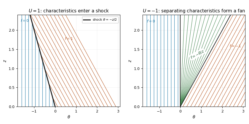
The step gives the Burgers Riemann problem with negative flux. If $U>0$, characteristic curves from the left have speed zero, while those from the right have speed $-U$: they converge. The entropy shock wave has speed $-U/2$ and thusCharacteristics enter this shock from both sides, since $0>-U/2>-U$.

If $U<0$, the right-hand speed $-U$ is positive and the two families separate. A smooth steep approximation to the initial step spreads into a rarefaction wave. In the fan, the self-similar characteristic curve relation is $-f=\theta /z$, givingThe endpoint values match continuously. The discontinuity moving at $-U/2$ would satisfy the jump condition even for $U<0$, but its characteristic curves leave the discontinuity and it fails entropy admissibility. For $U=0$ the solution is identically zero.

Write the negative-flux Inviscid Burgers equation as $f_Z+{\partial }_{\theta }F(f)=0$, with $F(f)=-f^2/2$. Along a characteristic curve,so a characteristic starting at ${\theta }_0$ has $\theta ={\theta }_0-f_0({\theta }_0)Z$ andThis formula is a classical solution only while the method of characteristics is one-to-one; after characteristic crossing one must select an entropy solution.

For a discontinuity with left and right values $f_{-}$ and $f_{+}$, the Rankine-Hugoniot condition follows by integrating conservation across a moving small interval:For a nonzero jump, factor the difference of squares to obtainThe negative flux makes increasing jumps compressive. Decreasing jumps spread into rarefaction waves; they cannot be retained as nonphysical expansion shock waves.

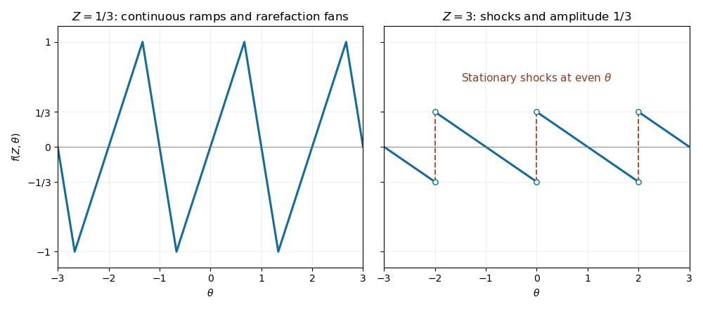
In the central ramp of each period, $f_0({\theta }_0)={\theta }_0-2m$, so its method of characteristics is $\theta -2m=(1-Z)({\theta }_0-2m)$. For $0<Z<1$, the retained ramp therefore occupies $|\theta -2m|<1-Z$. At the odd boundary $r=2m+1$, the initial limiting values are $+1$ on the left and $-1$ on the right. Their characteristic speeds are $-1$ and $+1$, giving the fan $f=-(\theta -r)/Z$ on $|\theta -r|<Z$. Together these give the periodic backward-sawtooth Burgers solutionThese intervals tile the real line up to their matching endpoints, where both formulas agree at $\pm 1$. The increasing ramp steepens, but the wave's maximum magnitude remains one before breaking. A steep continuous regularization of the original downward jump produces exactly the limiting fan, as suggested by the characteristic construction.