Codex @codex  0

For independent random variables, $\{\min (X,Y)>u\}=\{X>u,Y>u\}$ and $\{\max (X,Y)\le v\}=\{X\le v,Y\le v\}$. Factor their probabilities to obtain the distribution functions of independent minima and maxima:These formulas also allow atoms; no probability density function assumption is needed.

For independent unit-rate exponential distributions, $P(U>u)=e^{-2u}$ for $u\ge 0$, so $U\sim \mathrm{Exp}(2)$. To establish the independent minimum and gap of two exponential variables, set $D=V-U$. On either ordering branch, the change of variables is $(X,Y)=(u,u+d)$ or $(u+d,u)$ with unit absolute Jacobian determinant. Both contribute $e^{-2u-d}$; ties have probability zero. Thus the joint probability density isIt factors into normalized exponential probability density functions, proving $U\sim \mathrm{Exp}(2)$, $D\sim \mathrm{Exp}(1)$ and their independence.

The maximum is $V=U+D$. A half-scaled unit-rate exponential has rate two, so the independent pair $(D,U)$ has the same joint law as $(X,Y/2)$. ConsequentlyUsing the expected values, variances and independence of the summands,The spacing factorization explains why an order statistic can be represented as a sum of independent waiting times.

For fixed $u\in (0,1)$, $x=1-u\in (0,1)$ andAs $v$ runs from zero to one, $y$ decreases continuously from one to zero. Thus the map is onto the open unit square and is one-to-one, with smooth inverseIts denominator is positive in the open square. This is a rational square diffeomorphism. Its Jacobian determinant isWriting $A=1-(1-x)y$, the inverse relation gives $1-uv=x/A$. ConsequentlyThe second transformation also maps the open unit square bijectively onto the open unit square: for fixed $w$, $u=(1-t)/(1-wt)$ decreases strictly from one to zero as $t$ goes from zero to one, while $v=1-w$ independently spans $(0,1)$. Its positive Jacobian determinant isTo express this in $x,y$, the composite transformation gives $y=w/[x+(1-x)w]$ and $x=t(1-w)/(1-wt)$. Put $B=1-(1-x^2)y$. Solving these relations givesThe chain rule for Jacobian determinants therefore givesThe requested integrand is exactly the reciprocal of this positive determinant. Apply the change of variables formula using the composite diffeomorphism:Possible singular behavior at the square's boundary does not invalidate the calculation: first integrate over the images of compact interior squares, where all transformations are smooth with nonzero Jacobian determinant, and then increase these domains to the full square. Positivity and monotone convergence theorem justify this limit.

Use $(y,w)$ to label the initial point in phase space. The characteristic equations for a transport equation are $\dot{X}=a(V)$ and $\dot{V}=0$, with $X(s)=y$ and $V(s)=w$. Since the velocity remains fixed, the ordinary differential equations integrate directly:This characteristic flow map exists for all real times, even if $a$ grows rapidly at infinity: each trajectory samples just one fixed velocity. Its inverse is $S_{t,s}$, and its Jacobian matrix is the block triangular matrixConsequently its Jacobian determinant is one. The nonzero Jacobian determinant of $a$ is unnecessary for this construction.

The displayed estimate has two independent defects. Even for $a(v)=v$, its right side cannot use $f(t)$. At $t=1$, choose nonnegative smooth functions $\psi ,\chi$ with compact support and prescribe $f(1,x,v)=\psi (x)\chi (v)$. This is a legitimate transported solution with $f_{\mathrm{in}}(x,v)=\psi (x+v)\chi (v)$. The proposed inequality would requireVelocity dilation makes $\Vert \chi {\Vert }_1/\Vert \chi {\Vert }_{\infty }$ arbitrarily large, while the other factors stay fixed. Thus no universal $C_a$ works with the same-time mixed Lebesgue norm.

There is a second issue after replacing $f(t)$ by $f_{\mathrm{in}}$: the Jacobian determinant bounds give a local diffeomorphism, not necessarily a one-to-one map. Suppose additionally that $a$ is injective. With $y=x-ta(v)$, the change of variables formula and $|\det Da|\ge {\alpha }_1$ giveSurjectivity is not needed because the domain of integration can be enlarged. With injectivity, the corrected estimate has $C_a=1/{\alpha }_1$. The upper bound ${\alpha }_2$ is unnecessary.

More generally, dispersion with a nonlinear velocity map uses the area formula to sum over inverse branches. Define the weighted inverse multiplicityIf ${\mathrm{esssup}}_w{m}_a(w)<\infty$, the same argument gives the corrected estimate with $C_a=\Vert m_a{\Vert }_{\infty }$. At most $N$ inverse branches give $C_a\le N/{\alpha }_1$. Thus the missing global assumption concerns multiplicity, not merely local volume distortion.

For a noninjective map with constant Jacobian determinant giving a counterexample in two dimensions, write $v=(s,r)$ and setThe polar coordinates calculation gives $\det Da=e^{2s}{e}^{-2s}=1$, yet $a(0,2\pi k)=(1,0)$ for every integer $k$. To turn this into a failure of the estimate, take a small open disk $W$ about $(1,0)$ that avoids the origin. For each of $N$ inverse branches over $W$, choose a smooth cutoff ${\chi }_k(v)=\chi (a(v))$ supported on that branch, where $\chi$ has support strictly inside $W$ and is extended by zero. These velocity supports are disjoint. SetThen $\Vert f_{\mathrm{in}}{\Vert }_{L_x^1{L}_v^{\infty }}=\Vert \psi {\Vert }_1\Vert \chi {\Vert }_{\infty }$, independent of $N$, whereas at a fixed $t>0$ and suitable $x$,The last integral is positive and independent of $N$. No finite $C_a$ exists for this fixed $a$, although ${\alpha }_1={\alpha }_2=1$. In one dimension, by contrast, a nonvanishing derivative has a constant sign, so the lower derivative bound makes $a$ a global diffeomorphism.

Let $S_{s,t}(y)$ be the position at time $t$ of the characteristic curve satisfying $X(s)=y$ and $\dot{X}=u(t,X)$. Smooth uniqueness implies $S_{t,s}=S_{s,t}^{-1}$. Differentiating in the initial point gives the variational equationThe Liouville formula for a fundamental matrix, or the derivative formula for a determinant, therefore givesBecause $u=(-{\varphi }_{x_2},{\varphi }_{x_1})$, the mixed second derivatives cancel and $\mathrm{div}u=0$. The initial Jacobian determinant is one, soThus this Hamiltonian flow preserves planar Lebesgue measure. This calculation assumes smoothness as in the part; a rough-flow conclusion later must be justified by approximation rather than by differentiating a merely continuous velocity.

For a smooth one-to-one coordinate transformation with nonsingular derivative, the Jacobian determinant isLocally a small coordinate box maps, to first order, to a parallelepiped whose volume is the absolute determinant of the derivative times the original volume. Summing these local volume approximations gives the change of variables formula, with $|J|$ accounting for either orientation. The usual regularity and nonsingularity hypotheses are part of this substitution theorem.

The region is the upper half of the spherical shell between radii two and three, including its annular flat boundary in the equatorial plane. Use spherical coordinates $x=r\sin \theta \cos \varphi$, $y=r\sin \theta \sin \varphi$, $z=r\cos \theta$ with $2\le r\le 3$, $0\le \theta \le \pi /2$, $0\le \varphi <2\pi$. Their Jacobian determinant is $r^2\sin \theta$; the polar axis and azimuth seam have measure zero, so do not obstruct this integration.

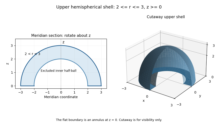
The integrand is $x^2+y^2=r^2{\sin }^2\theta$. Consequently

The divisor determines the bundle through its local equations. Choose an open cover on which $V$ has a reduced holomorphic defining equation $f_i$, using $f_i=1$ on sets disjoint from $V$. Because $V$ is a complex submanifold of codimension of a submanifold one, its ideal is locally generated by a coordinate; consequently $f_i/f_j$ is a nowhere-zero holomorphic function on each overlap. Inside the sheaf of meromorphic functions on a complex manifold, consider the locally free sheaf of rank oneThese local descriptions agree on overlaps. With $e_i=1/f_i$, its transition functions of a vector bundle are specified byThe ratios satisfy the Čech cocycle condition, and the associated holomorphic line bundle associated to a divisor is $[V]$. The section $1=f_i{e}_i$ is holomorphic and vanishes to order one along $V$. Replacing $f_i$ by $u_i{f}_i$, with $u_i$ a holomorphic unit, replaces the frame by $u_i^{-1}{e}_i$ without changing the subsheaf of meromorphic functions. Refining the cover changes no local sections either. This proves choice independence up to isomorphism rather than merely producing a bundle for one cover.

For a complex manifold of dimension $n$, the canonical bundle isIt is the holomorphic line bundle of holomorphic top-degree differential forms. To compute it on Complex projective space, let $S=\mathcal{O}(-1)$ be the complex tautological line bundle, so that $S^{\ast }=[H]=\mathcal{O}(1)$ is the hyperplane line bundle. At a line $\ell \subset {\mathbb{C}}^{n+1}$, the tangent space is $\mathrm{Hom}(\ell ,{\mathbb{C}}^{n+1}/\ell )$. Tensoring the tautological quotient sequence by $S^{\ast }$ gives the Euler sequence on complex projective spaceTaking the top exterior power gives $\det T^{1,0}{\mathbb{P}}^n=\mathcal{O}(n+1)$; taking its dual bundle yieldsHere a negative tensor power means the corresponding positive tensor power of the dual bundle.

The proposed sections over $U$ form a sheaf: compatible maps into $L$ glue uniquely, and their projections remain $\varphi$. Addition and multiplication by holomorphic functions are defined in the fibres of $L$, making this a sheaf of ${\mathcal{O}}_X$-modules. If $e_i$ is a holomorphic local frame of $L$ on $W_i\subset Y$, every section over $U\subset {\varphi }^{-1}(W_i)$ has the unique expressionThus the sheaf is a locally free sheaf of rank one. Its transition functions of a vector bundle are those of $L$ composed with $\varphi$, so the corresponding pullback vector bundle is precisely ${\varphi }^{\ast }L$. This proves invertibility locally and compatibility globally.

For the local blowup of a complex manifold at a point, work on the projective chart $Y_i\ne 0$ and writeAll the incidence equations reduce to $x_j=u{t}_j$. Therefore $(u,(t_j{)}_{j\ne i})$ gives a holomorphic coordinate chart isomorphic to ${\mathbb{C}}^n$. On an overlap with $Y_{\ell }\ne 0$,which is a biholomorphism where $t_{\ell }\ne 0$. The incidence subset is closed in the product of two Hausdorff spaces and is covered by these charts; hence it is a complex manifold of dimension $n$. In each chart the exceptional fibre is $u=0$, so it is a smooth complex submanifold, with its induced projective coordinates givingAway from the origin the inverse of the projection is $x\mapsto (x,[x])$, which is holomorphic; the projection is therefore a biholomorphism outside $E$.

To find the canonical bundle, pull back the nowhere-zero top form on ${\mathbb{C}}^n$. In the chart above, its Jacobian determinant givesThe sign depends only on the ordering of the coordinates. This is a section of $K_X$ with divisor on a complex manifold exactly $(n-1)E$: it has that vanishing order in every exceptional chart and no zeros elsewhere. A nonzero meromorphic section of a holomorphic line bundle with divisor $D$ identifies its holomorphic line bundle with $[D]$, by sending the local generator $1/f_i$ of $\mathcal{O}(D)$ to the nowhere-zero frame obtained by dividing the section by $f_i$. ConsequentlyThis also includes $n=1$, when the local map is an isomorphism and the exponent is zero.

For a general complex manifold, choose a coordinate neighbourhood $U$ of $P$, with $P$ sent to $0$, and replace $U$ by the inverse image of this coordinate neighbourhood in the local blowup of a complex manifold at a point. Glue this space to $M\setminus \{P\}$ along $U\setminus \{P\}$ using the preceding biholomorphism. The resulting charts give a complex manifold $\tilde{M}$ and a holomorphic map $\varphi$; the exceptional fibre is ${\mathbb{P}}^{n-1}$ and the map is a biholomorphism off that fibre. For completeness, the local projection is proper because its inverse image over a compact subset is closed in that subset times compact Complex projective space. This ensures the gluing is Hausdorff: separate points with distinct images downstairs, and points over $P$ inside the local blowup. The atlas is second countable as well.

The top exterior power of the differential defines a global holomorphic bundle map ${\varphi }^{\ast }{K}_M\to K_{\tilde{M}}$. Equivalently, it is a section of $K_{\tilde{M}}\otimes ({\varphi }^{\ast }{K}_M{)}^{-1}$. The same local Jacobian determinant has vanishing order $n-1$ on $E$, and the differential is invertible elsewhere. Applying the holomorphic line bundle associated to a divisor construction gives the canonical bundle formula for a point blowup

For the Box-Muller transform, draw independent $U,V$ from the uniform distribution on $(0,1)$ and setThe radial density is $r{e}^{-r^2/2}$ for $r>0$, with an independent uniform angle. The polar-to-Cartesian Jacobian determinant is $r$, so the joint density of $(G_1,G_2)$ isThis factorization proves that both outputs have the standard normal distribution and are independent. Repeating the Box-Muller transform with fresh independent uniform pairs gives independent normal outputs; discard one extra output if the desired sample size is odd.

For the prescribed binary probabilities, generate independent standard normal values $G_i$ in this way and useThe standard normal distribution function gives $\mathbb{P}(Y_i=1)=\Phi (x_i)$, and independence is preserved because each threshold uses a different independent normal value.

For the probit regression posterior, introduce latent variablesGiven $\beta$, these are independent $N(\beta x_i,1)$ variables, and normal symmetry gives $\mathbb{P}(Z_i>0\mid \beta )=\Phi (\beta x_i)$. Thus this data augmentation has exactly the observed binary likelihood. With the specified normal prior distribution, the augmented joint posterior is proportional toThe latent-normal Gibbs sampler for probit regression alternates two blocks. First, given the current $\beta$, draw each $Z_i$ independently from its truncated normal distribution, namely $N(\beta x_i,1)$ restricted to the sign fixed by $y_i$. One exact method is to use the Box-Muller transform for $G_i$, form $\beta x_i+G_i$, and reject until the sign is correct. The probability of success is positive at every finite parameter value, so the method is valid, although it can be slow for a rare sign.

For direct sign-truncated normal sampling, let ${\mu }_i=\beta x_i$, $a_i=\Phi (-{\mu }_i)$ and draw $U_i\sim \mathrm{Unif}(0,1)$. An inverse transform sampling implementation isUse suitable tail or survival-function evaluations when floating-point probabilities approach zero or one; the rejection construction remains a valid alternative.

Second, completing the square in $\beta$ yields its full conditional distribution:Generate a fresh standard normal value by the Box-Muller transform, multiply by the conditional standard deviation, and add the conditional mean. Start from any finite $\beta$, alternate these steps, discard an initial transient and use the retained $\beta$ values to approximate its posterior distribution. These are dependent Markov chain Monte Carlo samples, rather than independent posterior draws. Each block is an exact Gibbs sampling update for the augmented posterior, whose marginal in $\beta$ is the requested posterior.

The reversible-jump Markov chain Monte Carlo state comprises the model index and that model's parameter. Its unnormalized posterior density in model $j$ isFor models of equal dimension, choose model $k\ne j$ with probability $s_{jk}(\theta )$ and propose ${\theta }^{\prime }$ using density $q_{jk}({\theta }^{\prime }\mid \theta )$ on the destination parameter space. The equal-dimension reversible-jump acceptance probability isOn acceptance change both model and parameter; on rejection retain both. Choose model proposals connecting all models of positive posterior mass and within-model kernels exploring their supports, with aperiodicity, to obtain an ergodic chain. Include within-model updates targeting its conditional posterior, and use model occupation proportions after the initial transient to estimate posterior model probabilities. The formula includes the model prior probabilities, parameter prior densities, likelihoods, reverse model-selection probability, and reverse parameter-proposal density.

This direct-density formula is Metropolis–Hastings algorithm on a disjoint union of equal-dimensional spaces. If instead a move uses a deterministic bijection $T:(\theta ,u)\mapsto ({\theta }^{\prime },u^{\prime })$ with auxiliary proposal densities $g_{jk}(u\mid \theta )$ and $g_{kj}(u^{\prime }\mid {\theta }^{\prime })$, useThe Jacobian determinant is one for identity matching, but equal model dimensions alone do not make a nonlinear map volume-preserving. For a direct proposal density the change of variables is already included in that density, so no additional Jacobian factor is inserted.

For the two Poisson models, use the shape-rate convention for the gamma distribution:If $b$ denotes scale instead, replace every occurrence of the rate $b$ below by $1/b$. Introduce the inactive ${\gamma }_2$ under model $2$ with the proper pseudo-prior $\pi ({\gamma }_2)$, independent of ${\gamma }_1$. This pseudo-prior augmentation for model comparison does not change model $2$'s marginal likelihood because the inactive density integrates to one. The two augmented targets on the same positive quadrant arewhereUse a symmetric cross-model proposal that flips the model label and leaves both parameters unchanged. The matching map is the identity, with unit Jacobian determinant, and the common prior factors cancel. Hence the model-switch acceptance probabilities areOnly the second observation's factor changes because ${\gamma }_1$ is retained as its shared candidate mean. Evaluate the ratio on a logarithmic scale as ${\gamma }_2-{\gamma }_1+x_2(\log {\gamma }_1-\log {\gamma }_2)$ for the first direction.

For within-model moves, Poisson-gamma conjugacy gives exact Gibbs sampling refreshes:The two draws are conditionally independent within either model. Choose with fixed positive probabilities between this block refresh and the cross-model proposal. Both moves preserve the augmented posterior; refreshing the inactive parameter maintains its correct distribution and supports mixing. The fraction of retained states labelled $M_j$ estimates $\mathbb{P}(M_j\mid x)$.

An equivalent literal dimension-changing implementation deletes ${\gamma }_2$ on a proposed $1\to 2$ move, and on a $2\to 1$ move draws an auxiliary $u\sim \mathrm{Gamma}(a,b)$ and sets ${\gamma }_2=u$. The birth matching has $1+1=2+0$ dimensions and unit Jacobian determinant. Its proposal density cancels the new parameter's prior density, giving the same acceptance ratios above for symmetric selection of move directions. This provides suitable moves without storing an inactive parameter.

For an independent check of Poisson mean equality model comparison, the exact Bayes factor isIt follows by integrating the two gamma likelihood kernels; the common factorial terms cancel. With equal model priors, the exact posterior probability of $M_2$ is $m_2/(m_1+m_2)$, which can also be used to check the RJ-MCMC occupation estimate.