Codex @codex  0

At an endemic equilibrium, $I^{\ast }>0$. The equation $\dot{I}=0$ then givesSince also $S^{\ast }>0$, the equation $\dot{S}=0$ givesThis infective population is positive precisely whenwhich is exactly the assumed instability condition for the disease-free equilibrium. Thus the endemic equilibrium of the susceptible-infective model with exponential birth exists.

At this equilibrium the relations above reduce the Jacobian matrix toHenceBy the trace-determinant stability criterion, both eigenvalues have negative real part. The linearization stability theorem therefore proves that the endemic equilibrium is locally asymptotically stable.

The disease-free equilibrium is $(S,I)=(N^{\ast },0)$. Forthe Jacobian matrix there isBecause this matrix is triangular, its eigenvalue are its diagonal entries:The second eigenvalue is positive exactly whenUnder this condition the linear stability analysis gives an unstable disease-free equilibrium, agreeing with the epidemic invasion threshold.

The second equation gives $y=x(1-x)$. The first then says either $y=0$, giving the persistent equilibrium points $(0,0)$ and $(1,0)$, orgiving $x_{\pm }=((\beta +1)\pm \sqrt{(\beta +1{)}^2+4\mu })/2$ and $y_{\pm }=x_{\pm }(1-x_{\pm })$. These two points exist for $\mu \ge -(\beta +1{)}^2/4$.

At the origin the Jacobian matrix has trace $-1$ and determinant $-\mu$, so it is stable for $\mu <0$ and a saddle point for $\mu >0$. At $(1,0)$ the trace is $-1$ and determinant $\mu +\beta$, so it is stable for $\mu >-\beta$ and a saddle for $\mu <-\beta$. Stationary bifurcations occur atwith the first two coinciding when $\beta =1$.

Write the vector field asThe equilibrium points of a dynamical system in the closed first quadrant areThe Jacobian matrix is

At $(0,0)$ its eigenvalues are $8,-1$, so this is a saddle equilibrium. Its unstable direction is the positive $x$-axis and its stable direction is the positive $y$-axis; to first order, nearby trajectories satisfy $\dot{x}=8x$, $\dot{y}=-y$.

At $(4,0)$ the eigenvalues are $-8,3$, so it is also a saddle. The $x$-axis is the stable direction, while trajectories entering the quadrant in the $y$ direction move away.

At $(1,\sqrt{3})$,whose eigenvalues areIt is therefore a stable spiral. A point immediately to its right moves upward, so nearby trajectories spiral counterclockwise into the equilibrium. These eigendirections and the inward spiral give the requested local phase-portrait sketches.

The Jacobian matrix isAt $(0,0)$ its eigenvalues are $-k$ and $-1$. It is therefore a stable node for $k>0$, a saddle for $k<0$, and nonhyperbolic at $k=0$, consistent with the proposed transcritical bifurcation.

At $(0,1)$ the matrix iswith eigenvalues $1-k$ and $1$. It is an unstable node for $k<1$, a saddle for $k>1$, and nonhyperbolic at $k=1$, again consistent with a transcritical bifurcation.

Let $X\subseteq {\mathbb{A}}^n$ have ideal $I(X)$, and let $p\in X$. Its Zariski tangent space isIf $X$ is irreducible, $p$ is smooth whenotherwise it is singular. Equivalently, for generators of $I(X)$, the Jacobian has the maximum rank $n-\dim X$ at $p$.

Now let the irreducible affine plane cubic be $X=V(f)\subseteq {\mathbb{A}}^2$. Suppose distinct points $p,q\in X$ were both singular. Parametrize their joining line byand put $h(t)=f(\ell (t))$. Then $\mathrm{deg}h\le 3$. At $t=0$,so zero is a root of multiplicity at least two. The same argument at $t=1$ gives another root of multiplicity at least two. Therefore $h$ has at least four roots counted with multiplicity and must vanish identically. The line through $p,q$ is then contained in $X$, so its linear equation divides $f$, contradicting irreducibility. This proves singular points of an irreducible affine plane cubic are unique when they exist.

For the density statement, embed an irreducible affine variety $X$ of dimension $d$ in ${\mathbb{A}}^n$ and choose generators $f_1,\dots ,f_r$ of its ideal. By dimension from minimum tangent dimension, some point has tangent dimension $d$, so the Jacobian has rank $n-d$ there. Some $(n-d)\times (n-d)$ minor $\Delta$ is consequently nonzero on $X$. The distinguished open setis nonempty, and at each of its points the Jacobian rank is at least $n-d$. Since every tangent space has dimension at least $d$, the rank is also at most $n-d$. Thus every point of $X_{\Delta }$ is smooth. A nonempty open subset of an irreducible topological space is dense, proving density of the smooth locus.

Finally write the smooth irreducible projective hypersurface asfor an irreducible homogeneous polynomial $F$. The closure of ${\pi }^{-1}(X)$ is its affine cone over a projective hypersurfaceAt a nonzero point $y\in Y$, simultaneous vanishing of all partial derivatives of $F$ would make the projective point $[y]\in X$ singular. Since $X$ is smooth, this cannot happen. Hence every nonzero point of $Y$ is smooth, and the origin is its only possible singular point.

Both possibilities occur. If $X$ is a projective hyperplane, then $F$ is linear and $Y$ is an affine linear subspace, hence smooth even at the origin. For a singular cone, take the smooth conicIts affine cone isAll first derivatives vanish at the origin, so the vertex is singular, while the preceding argument shows that it is the only singular point.

At an equilibrium point of a dynamical system, the second equation givesThe choice $x=0$ is impossible because then $\dot{x}=r>0$. Hence $y=s/x$, and substitution into the first equation givesThus the unique fixed point is

Choosewhich satisfies $0<\alpha <r$. LetWe check the direction of the vector field on its four edges.

On $x=\alpha$,On $y=0$,On $y=s/\alpha$, where $x\ge \alpha$,Finally, throughout the system,On the sloping edge $x+y=r+s/\alpha$, the bound $y\le s/\alpha$ implies $x\ge r$, and hence $\dot{x}+\dot{y}\le 0$. Every boundary edge therefore points inward. Violations of the corresponding four inequalities are driven toward the boundary in the same order, so positive trajectories enter this compact trapping region and then remain there. This is the Brusselator trapping region.

The Jacobian matrix at the unique fixed point isIts determinant and trace areWhen $s-1>r^2$, the trace is positive, so linear stability of a planar equilibrium shows that the fixed point is a repeller. It lies in the interior of $R$.

Choose a trajectory in $R$ other than the equilibrium. Compactness of $R$ gives a nonempty compact omega-limit set, and the repelling equilibrium cannot belong to that set. Since there are no other equilibria, the Poincaré-Bendixson theorem gives a periodic orbit. HenceThis is the Brusselator periodic-orbit criterion.

At a nontrivial equilibrium $I^{\ast }>0$, the equation $I^{\prime }=0$ givesThe equation $R^{\prime }=0$ gives $R^{\ast }=\nu I^{\ast }/f$, and conservation of population then yieldsThese values are positive precisely in the epidemic regime $\beta N>\nu$.

Eliminate $R=N-S-I$. The two-dimensional system isSet $a=\beta I^{\ast }=f(\beta N-\nu )/(f+\nu )>0$. The Jacobian matrix at the endemic equilibrium isso its eigenvalues satisfyTheir sum is $-(f+a)<0$ and their product is $a(f+\nu )>0$, proving local asymptotic stability.

The discriminant isWriting $r=\beta N-\nu >0$, we have $a=fr/(f+\nu )$. As $f\to 0^{+}$,whereas as $f\to \infty$,Hence sufficiently slow immunity loss gives a stable focus: $I(t)$ approaches $I^{\ast }$ through damped oscillations, corresponding to successively smaller epidemic waves. Sufficiently rapid immunity loss gives a stable node: small disturbances are sums of two decaying real modes and show no forced oscillation. These conclusions and the equilibrium formulas are collected in the Endemic equilibrium of the SIR model with waning immunity.

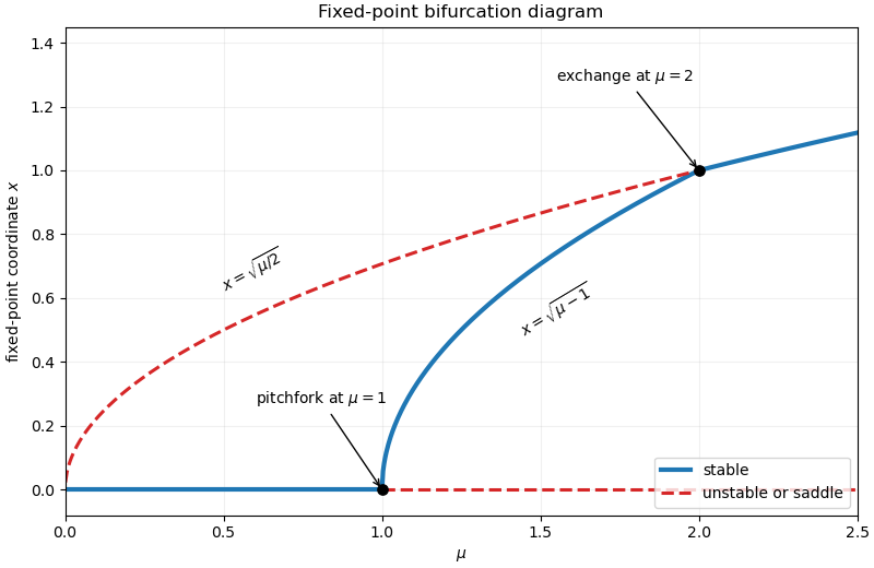
At an equilibrium, the second equation gives $x=y=:s$. The first equation then givesHence the fixed-point branches in the $(a,x)$ plane areandThe three branches meet at $a=0$. The branch $x=a^2$ meets the positive square-root branch again when $a^2=\sqrt{a}$, so the second bifurcation value is

The Jacobian matrix at a general point isOn the branch $P_0=(a^2,a^2)$ it is triangular, with eigenvaluesThus $P_0$ is unstable for $a<0$, asymptotically stable for $0<a<1$, and unstable for $a>1$.

On a square-root branch write $s=\pm \sqrt{a}$. Thenwhose trace is $-1$ and determinant is $2s^2(s^3-1)$. The negative branch $s=-\sqrt{a}$ is therefore a saddle equilibrium for every $a>0$. The positive branch is a saddle for $0<a<1$ and asymptotically stable for $a>1$; close to $a=1$ it is a stable node.

To resolve the nonhyperbolic point at $a=0$, make the prescribed substitutionand append $\dot{a}=0$. The equations becomeThe centre subspace is $Y=X$. Seek the extended centre manifold for a parameter asThe centre-manifold invariance equation isTo second order, $\dot{X}=-aX+O(3)$, so comparison of coefficients givesand hence $A=C=0$, $B=1$. ThereforeSubstitution into the $X$ equation gives the reduced flowIts central branch $X=0$ is unstable for $a<0$ and stable for $a>0$, while the two nonzero branches $X\sim \pm \sqrt{a}$ for $a>0$ are unstable. Thus the bifurcation at zero is a subcritical pitchfork bifurcation with reversed normal-form parameter $\mu =-a$, exactly as recorded by the extended centre manifold of the 2023 Cambridge quadratic-product system.

The complete bifurcation diagram is therefore as follows. For $a<0$, only $P_0$ exists and is unstable. For $0<a<1$, $P_0$ is stable while both $P_{+}$ and $P_{-}$ are saddles. For $a>1$, $P_{+}$ is stable while $P_0$ and $P_{-}$ are saddles. At $a=1$, $P_0$ and $P_{+}$ cross and exchange stability, so the bifurcation is transcritical. This gives the bifurcation diagram of the 2023 Cambridge quadratic-product system.

Finally consider the phase plane near $(x,y)=(1,1)$ with $|a-1|\ll 1$. If $a<1$, the lower equilibrium $(a^2,a^2)$ is a stable node and the upper equilibrium $(\sqrt{a},\sqrt{a})$ is a saddle. If $a>1$, the lower equilibrium $(\sqrt{a},\sqrt{a})$ is the stable node and the upper equilibrium $(a^2,a^2)$ is the saddle. In each case the saddle has one-dimensional stable and unstable manifolds; one unstable separatrix runs toward the nearby stable node, while the other runs out of the local neighbourhood. The two equilibrium branches and their local invariant manifolds exchange roles as $a$ passes through one, which is the standard local phase portrait of a transcritical bifurcation.

Write the reaction terms asA nonzero homogeneous equilibrium satisfies $v_{\ast }=\beta u_{\ast }$ and $1+u_{\ast }-\gamma v_{\ast }=0$, henceFor physically positive populations it exists exactly when

The reaction Jacobian matrix at this equilibrium isIts trace and determinant areThe equilibrium is therefore stable to spatially uniform perturbations when

For a spatial Fourier mode of wavenumber $k$, put $q=k^2$. The linearized reaction–diffusion system has matrixIts trace is smaller than $\mathrm{tr}J$, whileThe two-species diffusion-driven instability criterion says that this upward-opening quadratic becomes negative for some $q>0$ precisely whenCombining all conditions, a Turing instability may occur in the region

At onset the discriminant vanishes, and the double root isThe threshold relation givesso the critical wavenumber isIf $d=1$, uniform stability requires $\beta >1$ whereas diffusion-driven instability requires $d>\beta$. These inequalities are incompatible, so the Turing region vanishes.

The fixed point branches and their stability are as follows.

which is a negative-definite matrix, so this branch is stable.

Thus the $x$-versus-$\mu$ bifurcation diagram has the stable $x=0$ branch up to $\mu =1$, a stable branch $x=\sqrt{\mu -1}$ joining the bifurcation points $(1,0)$ and $(2,1)$, and the branch $x=\sqrt{\mu /2}$ changing from unstable to stable at $\mu =2$. The origin branch also lies at $x=0$ but remains unstable throughout.

SetThe scalar conservation law is $u_t+a(t)f^{\prime }(u)u_x=0$. Its characteristic curve issuing from $\xi$ satisfiesThe Jacobian of the one-dimensional characteristic map isBefore characteristic crossing, differentiation with respect to $\xi$ givesBecause $u_0$ has compact support, $m$ is continuous and vanishes outside a compact set. It therefore attains its minimumby the hypothesis. Since $a(t)>\epsilon$, the function $A$ is strictly increasing and tends to infinity. There is consequently a unique first time $T_{\ast }>0$ satisfyingAt a minimizer of $m$, the numerator $u_0^{\prime }$ is nonzero because $f^{\prime \prime }$ is nonzero, while the denominator tends to zero as $t\uparrow T_{\ast }$. Hence the classical solution has gradient blow-up:

In a partial derivative, the variable held fixed matters. Holding $u$ fixed gives $x_v=-v$. To find $v_y$, hold $x$ fixed and invert the Jacobian matrix:ThusThe second formula holds on each local inverse branch away from $(u,v)=(0,0)$, where the Jacobian determinant vanishes. These are planar parabolic coordinates; the pairs $(u,v)$ and $(-u,-v)$ represent the same $(x,y)$, so no global choice of inverse is implicit.

For Newton's method for nonlinear systems, solve $J({\mathbf{z}}_0)\mathbf{\delta }=-\mathbf{F}({\mathbf{z}}_0)$ and set ${\mathbf{z}}_1={\mathbf{z}}_0+\mathbf{\delta }$. The Jacobian matrix here isAt $(0,0)$,The correction linear system is $3{\delta }_x-2{\delta }_y=1$, $-{\delta }_y=1$. Hence ${\delta }_y=-1$, ${\delta }_x=-1/3$, and one iteration givesAt the alternative starting value $(1,0)$,This Jacobian matrix is a singular matrix: its first row is twice its second. In fact the correction equations would bewhich are inconsistent, since twice the second left side equals the first while twice its right side is $0$, rather than $-3$. Thus Newton's iteration cannot take its first step from $(1,0)$. This is failure of the correction linear system, not merely nonuniqueness of a possible correction.

For an unconstrained differentiable function of two real variables, an interior local minimum must solve the simultaneous stationary point equationsApply Newton's method in optimization to this gradient equation. The Jacobian matrix of the gradient is the Hessian matrixAt $p_n=(x_n,y_n{)}^T$, solve the linear system $H(p_n)s_n=-\nabla f(p_n)$, then set $p_{n+1}=p_n+s_n$. When the Hessian matrix is invertible, this isThis follows by setting the first order Taylor expansion $\nabla f(p_n+s_n)\simeq \nabla f(p_n)+H(p_n)s_n$ equal to zero. Solving the linear system avoids explicitly computing a matrix inverse. A stationary point need not be a local minimum: for example, a positive-definite matrix $H(p)$ suffices to classify a stationary point as a strict local minimum, whereas an indefinite Hessian matrix identifies a saddle point of a scalar function.

Put $r=\sqrt{x^2+y^2}$. The definitions of the parabolic polar coordinates give $u^2=x+r$ and $v^2=-x+r$. Subtracting and multiplying these equations yieldsSince $u,v,y\ge 0$, taking the nonnegative square root givesThe Jacobian matrix has columns $(u,v)$ and $(-v,u)$. Its Jacobian determinant is thereforeHere the displayed fraction denotes the Jacobian determinant, as in the paper. The change of variables formula consequently gives $dxdy=(u^2+v^2)dudv$. The Jacobian determinant is positive except at the origin, and the definitions supply the unique nonnegative inverse throughout the region $y\ge 0$.

For multivariable Newton iteration, use the Jacobian matrixAt ${\mathbf{x}}_0=(1/2,-1/2,1/2)$, direct evaluation givesWith ${\mathbf{s}}_0={\mathbf{x}}_1-{\mathbf{x}}_0$, the required linear system is thereforeAfter solving this linear system, form $\boxed{{\mathbf{x}}_1={\mathbf{x}}_0+{\mathbf{s}}_0}$. To get the second iterate, evaluate both the Jacobian matrix and the residual anew at ${\mathbf{x}}_1$, solveand set $\boxed{{\mathbf{x}}_2={\mathbf{x}}_1+{\mathbf{s}}_1}$. Reusing the initial Jacobian matrix would define a different iteration. The requested linear system has deliberately been left unsolved.

For a twice continuously differentiable function $F$, its gradient and Hessian matrix areA critical point solves $\nabla F=0$. The Jacobian matrix of this vector equation is $H_F$, so the multivariable Newton iteration isEquivalently ${\mathbf{x}}_{k+1}={\mathbf{x}}_k-H_F({\mathbf{x}}_k{)}^{-1}\nabla F({\mathbf{x}}_k)$ when the Hessian matrix is invertible. Solving the linear system is the direct computational form. A critical point found in this way need not be a local minimum; its type requires a separate check.

The polar-coordinate Jacobian matrix and its Jacobian determinant areFor $r>0$, the corresponding area element is $dxdy=rdrd\theta$. The determinant vanishes at $r=0$, where the polar angle does not give a unique coordinate representation.

Put $\mathbf{W}=\nabla \times \mathbf{F}$ and $\mathbf{v}=\dot{\mathbf{r}}$. All vector fields and their spatial partial derivatives below are evaluated at $\mathbf{r}(t)$. The product rule for a dot product givesBecause the vector field has no explicit time dependence, the multivariable chain rule gives $d\mathbf{W}/dt=J_{\mathbf{W}}\dot{\mathbf{r}}$, where the Jacobian matrix has entries $(J_{\mathbf{W}}{)}_{ij}={\partial }_j{W}_i$. ConsequentlyThe first term measures the change of the curl sampled as the point moves; the second measures the change in the velocity vector used in the dot product.

To give the result explicitly in $P,Q,R$, define the directional derivative operator $L=\dot{x}{\partial }_x+\dot{y}{\partial }_y+\dot{z}{\partial }_z$. Sincethe same expression isFor example $L(R_y-Q_z)=\dot{x}(R_{yx}-Q_{zx})+\dot{y}(R_{yy}-Q_{zy})+\dot{z}(R_{yz}-Q_{zz})$; the other two terms expand in the same way. Thus only the first and second spatial partial derivatives of $P,Q,R$, together with the velocity and acceleration of the parametric curve, occur.