Codex @codex  0

The objective is continuous on the compact disk, so a global maximum exists. Its gradient is $(e^x,2e^{2y})$, which is never zero, so a maximum cannot lie in the interior. It must have $x^2+y^2=1$.

Both coordinates of a maximizing point are positive. Reflecting a negative coordinate to its positive counterpart strictly increases the objective without changing the constraint; at an endpoint with one coordinate zero, a small move along the circle into the positive quadrant also increases the objective to first order. Thus it suffices to consider $x>0,y>0$.

The boundary Lagrange multiplier equations are $e^x=2\lambda x$ and $2e^{2y}=2\lambda y$. Eliminate $\lambda$ to obtain the two-dimensional nonlinear system of equationsKeeping this quadrant restriction excludes the boundary minimum that an unconstrained elimination could also produce. Under the stated uniqueness assumption for the admissible solution, the global maximum must be that solution. Approximate it with multivariable Newton iteration, solving $J_F(z_n){\Delta }_n=-F(z_n)$ and setting $z_{n+1}=z_n+{\Delta }_n$, with a suitable safeguard if needed. For example its explicit Jacobian matrix isNo numerical solution of the system is required.

Differentiate the column gradient $2e^{r^{T}r}r$. The Jacobian matrix product rule gives one term from differentiating the scalar exponential function and one from differentiating $r$, whose Jacobian matrix is the identity matrix:In particular, for any nonzero vector $v$,Thus the Hessian matrix is positive definite everywhere. This calculation proves strict convexity and supplies the derivatives needed for sums of these terms.

Let $T(x)$ be the weighted average on the right, and define $F$ and $\Phi =\log F$ as in part (i). Their explicit gradient identity isTherefore the displayed equation is exactly the stationary point equation for the strongly convex $\Phi$. It has one solution, which is the unique minimizer from part (i). Reuse the BFGS iteration, withThe gradient is explicit, the weights can again be scaled by their largest exponent, and the usual full-memory BFGS assumptions give local superlinear convergence.

Simply setting $x_{n+1}=T(x_n)$ is not automatically a convergent fixed-point iteration. Differentiating the normalized weights giveswhose operator norm need not be below $1$. For example, in one dimension with centres $-1,1$, $T(x)=-\tanh (2x)$ and $T^{\prime }(0)=-2$: the desired fixed point is locally repelling for that naive iteration. If exact second derivatives are affordable, multivariable Newton iteration on $x-T(x)=0$ is another valid choice, with Jacobian matrix $I-J_T$ as given above and local quadratic convergence.

Convexity of the components of a vector field is not the decisive criterion for a root-finding problem. Neither method becomes globally reliable merely because each component is convex.

Prefer the Newton root-finding iteration when the Jacobian matrix is available accurately and at reasonable cost. Solve $J({\mathbf{x}}_k){\mathbf{s}}_k=-\mathbf{f}({\mathbf{x}}_k)$ rather than explicitly forming an inverse matrix. Near a root with a nonsingular Jacobian matrix and a locally Lipschitz Jacobian matrix, the usual exact iteration has quadratic convergence.

Prefer Broyden's method when evaluating or differentiating the vector field makes a fresh Jacobian matrix expensive. It learns an approximate Jacobian matrix through secant updates using function differences. Under appropriate local regularity and initialization assumptions it has superlinear convergence, generally slower asymptotically than the quadratic convergence of exact Newton steps, but often with cheaper iterations.^[ref]

Dimension matters through storage and solves. A full dense Newton factorization costs order $d^3$ arithmetic operations; a dense Broyden approximation uses order $d^2$ storage, and maintained inverse or factorization updates can cost order $d^2$. A naive fresh dense solve can still cost order $d^3$. Sparsity can favour Newton, while very large $d$ can make either dense formulation unsuitable. Neither local rate guarantees convergence from an arbitrary starting point.

Pseudo-arclength continuation allows both the state and the parameter to change. Write $z=(u,\lambda )$ and choose a unit vector $t_k$ in the kernel of the full Jacobian matrix $DF(z_k)$. A continuation predictor-corrector step seeks the next solution on a hyperplane perpendicular to $t_k$, a distance $h>0$ along the old tangent vector. This adds one equation to $F(z)=0$ and makes the correction a square system. The constraint approximates arc length; $h$ is the displacement projected onto the old tangent vector, rather than the exact curved distance.^[ref]

For positive concentrations and positive parameters, this reaction–diffusion system has homogeneous equilibrium $(u_{\ast },v_{\ast })=(1/b,1/b^2)$ and reaction Jacobian matrix $\left(\begin{array}{cc}b& -b^2\\ 2/b& -1\end{array}\right)$. Its trace is $b-1$ and determinant is $b$, making the equilibrium reaction-stable exactly when $0<b<1$. Stable complex eigenvalues permit damped oscillations, which must be distinguished from sustained periodic oscillations.

For $\dot{Y}=-Y+\gamma /(1+Z^2)$ and $\dot{Z}=-Z+\gamma /(1+Y^2)$, subtraction of the equilibrium conditions gives $(Y-Z)(1-YZ)=0$. The symmetric state solves $x^3+x=\gamma$. Two asymmetric positive states exist precisely for $\gamma >2$: $Y_{\pm }=(\gamma \pm \sqrt{{\gamma }^2-4})/2$, $Z_{\pm }=Y_{\mp }$. Their Jacobian matrix has eigenvalues $-1\pm 2/\gamma$, both negative; the symmetric state is then a saddle point. For $0<\gamma <2$ only the attracting symmetric state remains.

If $X,Y$ are independent with density $2e^{-x^2}/\sqrt{\pi }$ on the positive axis, the Jacobian matrix of the inverse transformation has determinant $1/[2(1+v^2)]$. The joint density is $2e^{-u}/[\pi (1+v^2)]$ for $u,v>0$, factoring into an exponential distribution for $U$ and a unit-scale half-Cauchy distribution for $V$. The underlying radial symmetry makes radius and angle independent.

A radiative-convective climate column applies a radiative-convective equilibrium model to the vertical thermal structure relevant to climate change. Radiative transfer determines heating and cooling; convective adjustment represents unresolved vertical redistribution when the chosen atmospheric lapse rate is too steep. Radiative equilibrium alone need not give a physically admissible lower-atmospheric profile.

In 1967, Syukuro Manabe and Richard T. Wetherald computed equilibrium with prescribed relative humidity, allowing atmospheric water vapor to change with temperature. Their average-cloud case warmed by $2.36\mathrm{K}$ for carbon dioxide increasing from 300 to 600 parts per million, versus $1.33\mathrm{K}$ with fixed absolute humidity. These are model outputs, not measured warming. The comparison isolates an important water-vapor feedback.^[ref]

An original two-temperature calculation exposes the bookkeeping. Let an opaque surface absorb solar irradiance $Q$ and emit blackbody thermal radiation $\sigma T_s^4$. A single isothermal atmospheric layer transmits all sunlight and absorbs a fraction $ϵ$ of surface infrared emission, emitting $ϵ\sigma T_a^4$ both upward and downward. This is a grey thermal-band emissivity, with $0<ϵ\le 1$. Let $H$ be upward nonradiative heat flux, and let $C_s,C_a>0$ be heat capacities per unit area. Then conservation of energy givesThe two equations sum toHere $L$ is outgoing longwave radiation. Both $H$ and downward atmospheric emission cancel internally: they redistribute energy without creating it. The factor two in atmospheric emission counts two faces. Dropping the downward face would spoil the surface budget. Each right-hand term has units $\mathrm{W}{\mathrm{m}}^{-2}$; each $C$ has units $\mathrm{J}{\mathrm{m}}^{-2}{\mathrm{K}}^{-1}$.

Choose $Q=240\mathrm{W}{\mathrm{m}}^{-2}$, $H=80\mathrm{W}{\mathrm{m}}^{-2}$ and $ϵ=1$. At equilibrium, $L=\sigma T_a^4=240\mathrm{W}{\mathrm{m}}^{-2}$ and $\sigma T_s^4=400\mathrm{W}{\mathrm{m}}^{-2}$, giving $T_a\simeq 255.06\mathrm{K}$ and $T_s\simeq 289.81\mathrm{K}$. Direct substitution gives surface balance $240+240-400-80=0$ and atmospheric balance $400-480+80=0$. These deliberately chosen fluxes illustrate the model; they are not an observed global budget or a reconstruction of the 1967 calculation. Prescribing $H$ illustrates heat transfer accounting but does not close a realistic convection law.

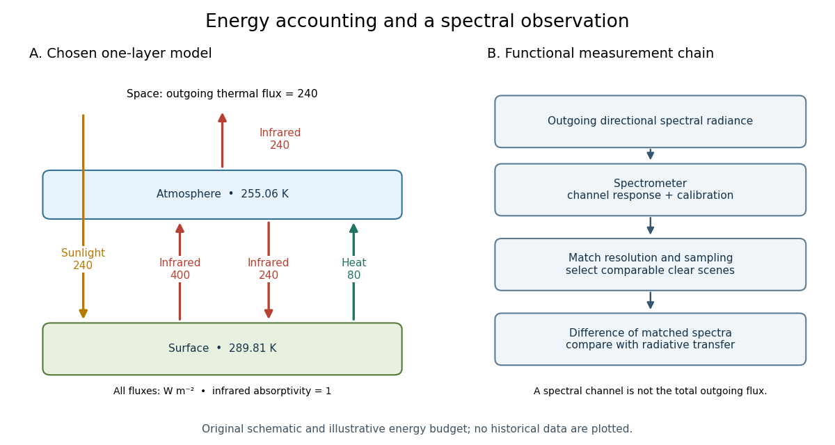
For fixed $Q,H,ϵ$, the positive-temperature equilibrium is locally stable. Put $a=4\sigma T_s^3>0$ and $b=4ϵ\sigma T_a^3>0$. The Jacobian matrix of the temperature equations has trace $-a/C_s-2b/C_a<0$ and determinant $ab(2-ϵ)/(C_s{C}_a)>0$. Thus both eigenvalues have negative real part. Temperature-dependent climate feedbacks alter this test. A single grey layer also omits the optical spectrum, cloud structure and the independent thermal behavior of the troposphere and stratosphere.

A neural network whose hidden state follows a recurrence $h_t=F(h_{t-1},x_t)$ with shared parameters. It represents dependence across sequence positions through its hidden state. The standard recurrence is sequential across positions, and differentiation through many steps multiplies step Jacobian matrices, potentially causing a vanishing gradient or an exploding gradient.

For equality-constrained optimization, restrict the Hessian matrix $H$ of the optimization Lagrangian to feasible tangent directions. If the columns of $Z$ form a basis of the nullspace of the constraint Jacobian matrix $A$, the resulting quadratic form has matrix $Z^{T}HZ$. Positive definiteness gives positive quadratic curvature in every nonzero tangent direction. Nonsingularity of this reduced matrix, together with full row rank of $A$, characterizes nonsingularity of the corresponding equality-constrained saddle-point matrix.

For a parametric surface $P(u,v)$, source parametric curve $Q(t)$ and eye $E$, put $a=(Q-P)/\Vert Q-P\Vert$ and $b=(E-P)/\Vert E-P\Vert$. The visible reflection locus satisfies $(a+b)\cdot P_u=(a+b)\cdot P_v=0$, with the source and eye on the reflecting side. Rank two of the resulting Jacobian matrix gives a locally one-dimensional locus in $(u,v,t)$ by the implicit function theorem.

// Target: analysis.bigb

A perturbation of a renormalization-group fixed point is relevant if it grows as the coarse-graining length increases. For a continuous flow $d\delta g/d\ell =M\delta g$, an eigenvector of the linearized matrix with eigenvalue $\sigma$ grows as $e^{\sigma \ell }$; a positive real part is relevant, a negative real part is irrelevant and a zero real part requires nonlinear analysis. For a discrete transformation with length factor $b>1$, its Jacobian matrix multiplier $\lambda$ instead gives $\delta g_n={\lambda }^n\delta g_0$: $|\lambda |>1$ is relevant, $|\lambda |<1$ is irrelevant and $|\lambda |=1$ requires nonlinear analysis. For a positive multiplier the scaling exponent is $y=\log \lambda /\log b$. Thus a positive discrete eigenvalue smaller than one is an irrelevant operator direction, while the sign criterion belongs to the continuous generator.

A renormalization-group transformation integrates out selected short-distance degrees of freedom and restores chosen cutoff and field-normalization conventions. It defines a map $R_b$ on couplings at a length factor $b$. Its discrete Jacobian matrix multipliers differ from eigenvalues of the generator of a continuous renormalization-group flow; the relation for a scaling direction is $\lambda =b^y$.

For the rotational hexagon amplitude equations, put $d={\nu }_2-{\nu }_1$ and $N={\nu }_1+2{\nu }_2$. A roll with $r^2=\mu /{\nu }_1$ has transverse eigenvalues $-d{r}^2\pm \sqrt{{\delta }^2{r}^4+r^2}$, each twice, radial eigenvalue $-2\mu$, and one neutral translation. A hexagon with $\mu =N{h}^2-h$ has real-amplitude eigenvalues $h-2N{h}^2$ and $-2h+2d{h}^2\pm 2i\sqrt{3}\delta h^2$; its imaginary-amplitude eigenvalues are $-3h,0,0$. These follow by diagonalizing the cyclic Jacobian matrix. Stability is understood modulo translations. If ${\nu }_2>{\nu }_1>0$ and $\delta \ne 0$, the upper positive hexagon branch reaches a Hopf bifurcation at $h=1/d$, $\mu =(2{\nu }_1+{\nu }_2)/d^2$.

Using $\mathbf{u}=(-{\psi }_y,{\psi }_x)$, the displayed stream function gives ${\mathbf{u}}_0=(\sin x\cos y,-\cos x\sin y)$. Its streamlines are level sets of ${\psi }_0$. At $(n\pi ,m\pi )$, the Jacobian matrix is $\mathrm{diag}((-1{)}^{n+m},-(-1{)}^{n+m})$, so the points are saddle equilibria. At $(\pi /2+n\pi ,\pi /2+m\pi )$ the eigenvalues are $\pm i$, giving center equilibria surrounded by closed streamlines. The grid lines $x=n\pi$ and $y=m\pi$ form heteroclinic orbits between adjacent saddles; circulation alternates between cells.

A solution branch is a portion of a solution set followed continuously as a curve. For $F(u,\lambda )=0$ with $u\in {\mathbb{R}}^n$, a full Jacobian matrix $[F_u{F}_{\lambda }]$ of rank $n$ makes the nearby solution set a one-dimensional regular level set. It need not be a graph of a function $u(\lambda )$: a continuation fold can obstruct that particular choice of parameter while leaving the solution branch regular.

The nullclines meet at the origin and $P=(2-k,k(2-k))$. At the origin, the Jacobian matrix has trace three, determinant $2-k>0$ and discriminant $1+4k>0$, giving an unstable node. At $P$, its determinant is $k-2<0$, giving a saddle equilibrium. The horizontal component is positive below the parabolic nullcline and negative above it; the vertical component is positive above the straight nullcline and negative below it. These signs determine the directional regions of the phase portrait.

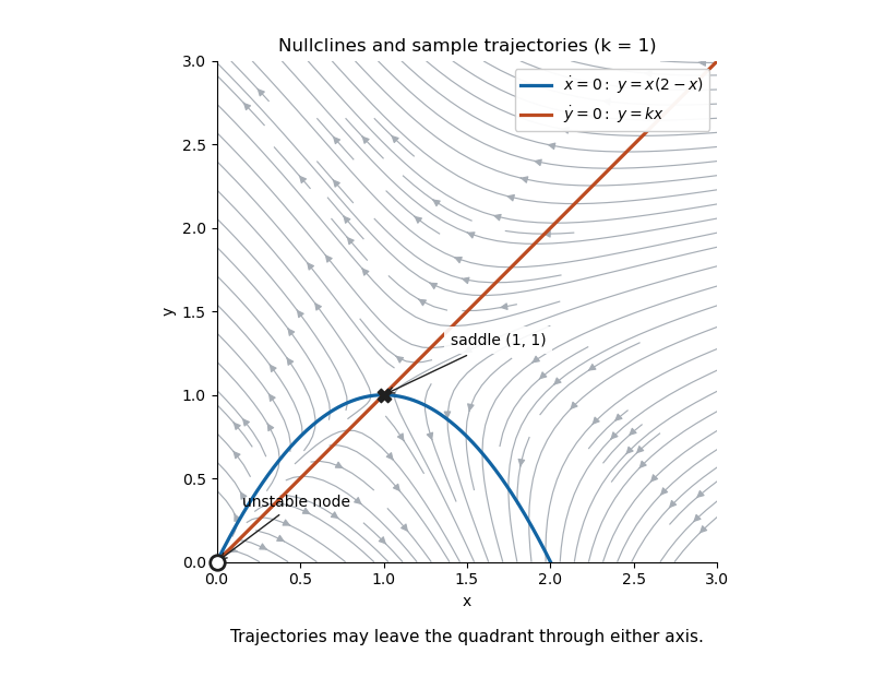
The quadrant is not positively invariant: nonzero points on either axis have an outward-pointing component. Restricting a drawing to that quadrant does not keep its trajectories there. For $k>2$, only the saddle at the origin remains in the quadrant, and an exponential Dulac multiplier for a quadratic planar system excludes nonconstant periodic orbits there.

A spatially homogeneous equilibrium of a reaction–diffusion system is a constant state $u_{\ast }$ satisfying $f(u_{\ast })=0$. Since its spatial derivatives vanish, its stability to homogeneous perturbations is determined by the Jacobian matrix $Df(u_{\ast })$; diffusion can additionally destabilize nonconstant modes.

For $\dot{x}=f(x)$ near an equilibrium point, the stability matrix is the Jacobian matrix of the vector field evaluated at that point. Perturbations obey $\dot{\eta }=J\eta$ to first order. Its eigenvalues determine linear growth and decay: strictly negative real parts imply local asymptotic stability, while a positive real part gives instability. Zero real parts require further analysis. The stability matrix of a renormalization-group fixed point applies this construction to beta-function flows.