Codex @codex  0

On the interior of the support $b<m$, differentiating the joint distribution of Brownian motion and its running maximum gives the joint probability densityMake the change-of-variables formula for a probability density $y=m$ and $z=m-b$. Its inverse is $m=y$, $b=y-z$, and its Jacobian determinant has absolute value one. Since $2m-b=y+z$, for $y,z\ge 0$ this yields

Apply the same dimensionless transformation independently to the two cups, giving $X,Y\in [-\pi /2,\pi /2]$. The total-volume condition becomes $X+Y\ge \pi /2$. Since neither variable can exceed $\pi /2$, this region has $0\le X\le \pi /2$ and $\pi /2-X\le Y\le \pi /2$, the triangle shown above.

By independence of random variables, the joint probability density is $\frac{1}{4}\cos x\cos y$. The desired double integral isThusBoundary equality has probability zero for these continuous random variables.

The support condition $-y<x<y$ forces $y>0$. As a check, the joint probability density integrates toFor any real $x$, the marginal density of $X$ isDividing the joint probability density by this marginal density gives the conditional density:Thus, conditionally on $X=x$, $Y-|x|$ has the rate-two exponential distribution.

For $U=X^2$, use the two inverse branches $x=\sqrt{u}$ and $x=-\sqrt{u}$. Each branch has absolute Jacobian determinant $1/(2\sqrt{u})$. Both lie in the original support exactly when $u>0$ and $y>\sqrt{u}$. The change of variables for probability densities therefore yieldsNo atom of a measure is created at $u=0$, since $\mathbb{P}(X=0)=0$. The value of the probability density function at this boundary may be assigned arbitrarily. Checking the integral over $0<u<y^2$ gives $4y{e}^{-2y}$, which integrates to one.

For a Borel set $A\subseteq \mathbb{R}$, the joint probability density givesFor each $x\ne 0$, substitute $z=xy$. The change of variables for probability densities contributes $dy=dz/|x|$, with the absolute value accounting for the reversed orientation when $x<0$. The line $x=0$ has two-dimensional Lebesgue measure zero, so omitting it changes no probability. By the Tonelli theorem,The bracket is nonnegative and its integral over $\mathbb{R}$ is one. This proves the probability density of a product of random variables formula:As usual, a probability density function is determined only almost everywhere; exceptional infinite values are harmless.

For the independent random variables with the specified uniform distribution, $f(x,y)=b^{-2}$ on $(0,b{)}^2$ and zero elsewhere. When $0<z<b^2$, the conditions $0<x<b$ and $0<z/x<b$ are equivalent to $z/b<x<b$. ThereforeThe value assigned at zero is arbitrary. Substitution $s=z/b^2$ checks normalization of a probability distribution: ${\int }_0^1-\log sds=1$. This is the product of independent uniform random variables law.

For the proposed joint probability density $\rho$, define the acceptance indicator functionOn the proposal's support the importance weight is $\pi (Y_i,V_i)/\rho (Y_i,V_i)=M{A}_i$. Therefore the requested augmented-space importance sampling estimator isIts expected value is $\theta$, provided ${\mathbb{E}}_p|\varphi (X)|<\infty$. This is not the ordinary estimator $n^{-1}{\sum }_{i}w(Y_i)\varphi (Y_i)$ from question 1. Taking the conditional expectation of this augmented estimator given all $Y_i$ produces that ordinary estimator, because $\mathbb{E}[A_i\mid Y_i]=w(Y_i)/M$. This is the Rao-Blackwell identity for a fixed-denominator rejection estimator.

Integrating the joint probability density over the auxiliary coordinate, as in (i), gives the marginal distributionIn particular, augmenting with $U$ preserves the target probability distribution of $X$. The other marginal distribution, though not needed to identify $X$, is ${\pi }_U(u)=M{\int }_{\Omega }q(x)1_{\{w(x)\ge Mu\}}dx$ for $0<u<1$. It need not be a uniform distribution on $(0,1)$.

Write $w=p/q$ where $q>0$, assigning zero elsewhere. The envelope ensures $0\le w/M\le 1$, and $\pi$ is nonnegative. Integrating its joint probability density over the auxiliary coordinate givesConsequently ${\int }_{\Omega }{\int }_0^1\pi (x,u)dudx={\int }_{\Omega }p(x)dx=1$. This proves normalization of a probability distribution; the change of integration order is justified by Tonelli's theorem.

The coordinates are generally dependent. For $p(x)>0$, their conditional probability density isThus $U\mid X=x$ has a uniform distribution on an interval whose endpoint depends on $x$. They are independent exactly when $w(x)$ is constant for $p$-almost every $x$, since only then do these conditional laws agree. In particular, $p=q$ is an exception: $X\sim p$ and $U\sim \mathrm{Unif}(0,1/M)$ are independent. An unconditional answer that they can never be independent would therefore be too strong.

By independence, the joint probability density is the product of the two uniform distribution densities:Changing its values on the boundary does not affect any probability or expected value.

If $(X,Y)$ has a joint probability density $f$, the product has the displayed probability density function, interpreted almost everywhere. For fixed $x\ne 0$, substitute $z=xy$ in the integral defining $\mathbb{P}(XY\in A)$; the absolute Jacobian determinant is $|x|$. The Tonelli theorem then exchanges the nonnegative integrals. The line $x=0$ has two-dimensional Lebesgue measure zero, so its omission creates no probability mass. A density may be infinite at exceptional points without creating an atom.

For independent $U,V$ uniform on $[0,1]$, real roots occur on $U\le V^2$, a region of probability $1/3$. On that region both roots are nonpositive. Both lie in $[-1,0]$ exactly when $\max (0,2V-1)\le U\le V^2$. Its area is $1/12$, so the conditional probability of both absolute values being at most one is $1/4$. Joint probability density integration turns algebraic discriminant and root constraints into simple planar areas.

The Rayleigh distribution is the probability distribution of the Euclidean norm of a two-dimensional random vector with independent zero-mean normal random variables of equal variance as components. If $X,Y\sim N(0,{\sigma }^2)$ are independent, thenHere $\sigma$ is the standard deviation of each component, not of the radius $R$. At $\sigma =1$ this gives the unit-scale probability density function $r{e}^{-r^2/2}$.^[ref]

This geometry turns two signed errors into one nonnegative distance. For example, suppose horizontal and vertical positioning errors are independent $N(0,4{\mathrm{cm}}^2)$ random variables. Their means both vanish, but the distance from the intended point is usually positive. The Rayleigh distribution with $\sigma =2\mathrm{cm}$ gives the probability of landing inside any centered disk. These are chosen model assumptions, rather than measurements of a particular instrument.

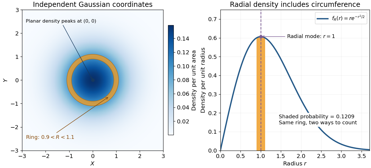
An apparently paradoxical feature is that the most likely location per unit area is the origin, while the radial mode is $\sigma$. A narrow annulus farther out has more area. Near zero that growing circumference outweighs the falling planar density; farther out the exponential function wins. Distinguishing densities measured against different elements of area or length resolves the paradox.

The joint probability density of $X,Y$ isIn polar coordinates, $x=r\cos \theta$, $y=r\sin \theta$, and the absolute Jacobian determinant is $r$. Thus the joint density of radius and angle factors asIntegrating over angle gives the Rayleigh distribution. The same factorization shows that the angle has uniform distribution and is independent of the radius. This is a short change of variables argument: an annulus of width $dr$ has area $2\pi rdr$ to first order.

The assumptions are substantive. Unequal component variances give elliptical rather than circular density contours; a nonzero mean displaces the center. Even zero covariance and equal normal distributions do not suffice without independence. For an original counterexample, let $X\sim N(0,{\sigma }^2)$ and let $S$ be an independent Rademacher random variable. Put $Y=SX$. Then $Y$ has the same normal distribution as $X$, and $\mathrm{Cov}(X,Y)=\mathbb{E}[S{X}^2]=0$. Nevertheless, all points lie on $y=x$ or $y=-x$, and $R=\sqrt{2}|X|$ has densitywhich is positive at zero, unlike the Rayleigh distribution. This pair is not a Gaussian random vector.

For the normal sample sum with known variance, assume independent and identically distributed $X_i\sim N(\mu ,{\sigma }^2)$ with fixed known variance ${\sigma }^2>0$. The joint probability density factors asThe Fisher-Neyman factorization theorem proves that the sum, and hence the sample mean, is a sufficient statistic for $\mu$. Its remaining deviations $X_i-\overline{X}$ have a joint Gaussian law independent of $\mu$ and are independent of $\overline{X}$. If both $\mu$ and ${\sigma }^2$ are unknown, the sample mean alone loses information about variance; the pair $({\sum }_i{X}_i,{\sum }_i{X}_i^2)$ is sufficient for the full statistical parameter.

A discrete counterexample shows why a sample mean is not automatically sufficient for arbitrary statistical models. Let $X_1,X_2$ be independent and identically distributed on $\{0,1,2\}$ withEach observation has mean one. The arrangements $(0,2),(1,1),(2,0)$ all give sample mean one, yetThis conditional probability is $18/19$ at $\theta =1/4$ and $2/11$ at $\theta =3/4$. The conditional distribution therefore still depends on the unknown statistical parameter: this sample mean is not a sufficient statistic. The useful reduction depends on the family of full-data laws, even when its mean stays fixed.

Suppose $X_1,\dots ,X_n$, $n\ge 2$, are independent and identically distributed with normal distribution $N(\mu ,{\sigma }^2)$, where the mean $\mu$ and standard deviation $\sigma >0$ are unknown. Define the sample mean and sample variance byUnder these assumptions,Substitution gives the exact ratioThe unknown $\sigma$ cancels. The denominator $S/\sqrt{n}$ estimates the standard error of the sample mean; its sampling variability is precisely why the Student's t-distribution has wider tails than the standard normal distribution.

The crucial independence has a geometric explanation. Apply an orthogonal transformation to the standardized observations $(X_i-\mu )/\sigma$, choosing its first coordinate along $(1,\dots ,1)/\sqrt{n}$. That coordinate is $Z$; the remaining $n-1$ coordinates are independent standard normal random variables whose squared sum is $V$. Their joint probability density factorizes because the transformation preserves the squared length. This also explains the loss of one statistical degree of freedom when estimating the mean. Uncorrelatedness alone would not establish the required independence for arbitrary data.

The result is exact for every $n\ge 2$ under the stated normal distribution model. A small sample size by itself does not justify it: a sample from an arbitrary probability distribution need not have the displayed chi-squared distribution or the necessary independence.