Studentized normal sample mean ($T=(\bar{X}-\mu )/(S/\sqrt{n})\sim t_{n-1}$)

Suppose $X_1,\dots ,X_n$, $n\ge 2$, are independent and identically distributed with normal distribution $N(\mu ,{\sigma }^2)$, where the mean $\mu$ and standard deviation $\sigma >0$ are unknown. Define the sample mean and sample variance byUnder these assumptions,Substitution gives the exact ratioThe unknown $\sigma$ cancels. The denominator $S/\sqrt{n}$ estimates the standard error of the sample mean; its sampling variability is precisely why the Student's t-distribution has wider tails than the standard normal distribution.

The crucial independence has a geometric explanation. Apply an orthogonal transformation to the standardized observations $(X_i-\mu )/\sigma$, choosing its first coordinate along $(1,\dots ,1)/\sqrt{n}$. That coordinate is $Z$; the remaining $n-1$ coordinates are independent standard normal random variables whose squared sum is $V$. Their joint probability density factorizes because the transformation preserves the squared length. This also explains the loss of one statistical degree of freedom when estimating the mean. Uncorrelatedness alone would not establish the required independence for arbitrary data.

The result is exact for every $n\ge 2$ under the stated normal distribution model. A small sample size by itself does not justify it: a sample from an arbitrary probability distribution need not have the displayed chi-squared distribution or the necessary independence.

Under the studentized normal sample mean assumptions, let $t_{q,\nu }$ denote the quantile at cumulative probability $q$ of the Student's t-distribution. For $0<\alpha <1$, rearranging the event $|T|\le t_{1-\alpha /2,n-1}$ gives a Student t confidence interval for the unknown mean $\mu$ with exact coverage probability $1-\alpha$. ^[ref]

Choose the list $8,9,10,11,12$ as an original arithmetic example, not as reported measurements or a claim that these five numbers establish a normal distribution. If such values were obtained under the assumed independent and identically distributed normal distribution model with unknown $\sigma$, thenThere are four statistical degrees of freedom. For a 95% confidence interval, $t_{0.975,4}=2.776445105\dots$, soUsing the standard normal quantile $z_{0.975}=1.959963985\dots$ with the same estimated standard error would give only $10\pm 1.385903824\dots$. That underestimates the correct margin by about 29.4%. Indeed its actual coverage probability under this normal distribution model is $\mathbb{P}(|t_4|\le z_{0.975})\simeq 0.8784$, rather than 0.95.

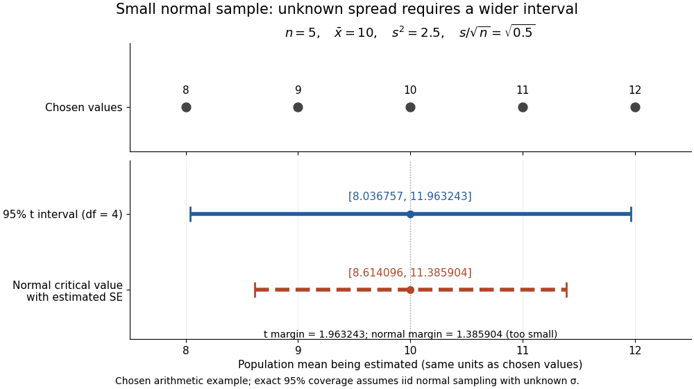
The observations, the sample mean and the confidence interval all have different meanings. The bar estimates the population mean; it is not an interval intended to contain 95% of individual observations. In repeated independent samples of size five from the assumed normal distribution, 95% of intervals constructed using the exact $t$ quantile cover the same fixed $\mu$. This is not a 95% posterior probability that the fixed statistical parameter lies in this particular realized interval. Such a probability requires a separate Bayesian inference model.

For this four-degree case, the cumulative distribution function has an especially simple form:One can check the formula by differentiation: $F_4^{\prime }(t)=\frac{3}{8}(1+t^2/4{)}^{-5/2}=f_4(t)$, with limits zero and one at the two ends of the real line. Solving the increasing equation $F_4(t)=0.975$ by the bisection method gives the quantile used above.