Codex @codex  0

 Incoming links: Multiplication

Abstract syntax tree precedence example Created 2026-10-13 Updated 2026-10-31

Consider Python programs x=2+3*4 and x=(2+3)*4. Operator precedence places multiplication inside the right operand of addition in the first abstract syntax tree. The parentheses instead place addition inside the left operand of multiplication in the second. Their right-hand sides evaluate to

2 + (3 \cdot 4) = 14

and

(2 + 3) \cdot 4 = 20

. No rule that simply reads all operators left to right would recover both structures. ^[ref]

Figure 1.
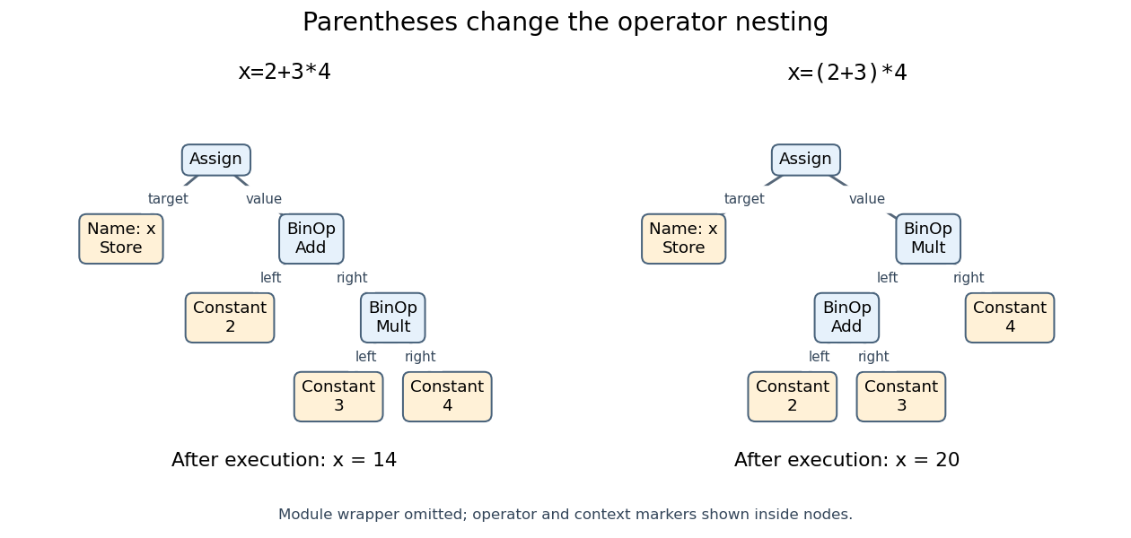
Two abstract syntax trees for variable assignment: operator precedence gives `x=2+3*4` the value $14$ , while parentheses give `x=(2+3)*4` the value $20$
. **Details**.

These are schematic views of Python trees: Module is omitted, and the Add/Mult and Store markers are written inside their owning nodes. In the actual schema, BinOp has left, op and right fields; Assign has a list of targets and a value. Name(id='x', ctx=Store()) marks the name as a variable assignment target. Reading x in a program expression instead uses Load. A variable assignment is a statement, not an equation asserting that two values are equal. ^[ref]

A restricted recursive evaluator can follow those fields. It accepts only integer literal values and binary addition, subtraction and multiplication; the surrounding variable assignment remains a separate action. Using type(value) is int excludes Boolean constants, even though Python treats bool as a subclass of int.

import ast

OPS = {ast.Add: lambda a, b: a + b,
       ast.Sub: lambda a, b: a - b,
       ast.Mult: lambda a, b: a * b}

def evaluate(node):
    if isinstance(node, ast.Constant) and type(node.value) is int:
        return node.value
    if isinstance(node, ast.BinOp) and type(node.op) in OPS:
        return OPS[type(node.op)](evaluate(node.left), evaluate(node.right))
    raise ValueError("outside the integer-expression language")

for source in ("x=2+3*4", "x=(2+3)*4"):
    tree = ast.parse(source, optimize=0)
    statement = tree.body[0]
    print(statement.targets[0].id, evaluate(statement.value))
# x 14
# x 20

The children in a rooted tree have ordered roles: left and right cannot be interchanged. For subtraction, 8-3 gives

5

while 3-8 gives

- 5

. Operator associativity also matters: 8-3-1 parses as (8-3)-1, giving

4

, whereas 8-(3-1) gives

6

. Here the syntax groups operators to the left; this does not assert the mathematical associativity of subtraction. Operator precedence determines grouping, rather than a general permission to reorder execution. For example, Python evaluates the calls in f()+g()*h() in the order f, g, h, although the multiplication result must be ready before the outer addition. ^[ref]

 Read the full article

Abstract syntax tree source location 2026-10-13

 View more

An abstract syntax tree can retain source locations even while omitting punctuation nodes. Python records one-based line numbers and zero-based UTF-8 byte offsets, with the end offset exclusive. In x=2+3*4, the multiplication node spans offsets

4

through

7

, and ast.get_source_segment returns 3*4. A copied location on a folded 12 describes the original span, not text newly present in the source. Such metadata supports error messages and editing tools without making an abstract syntax tree a lossless record of formatting. ^[ref]

// Target: computer-science.bigb

 Read the full article

Addition Created 2026-09-24 Updated 2026-10-13

 View more

Addition combines two numbers into their sum. For natural numbers, joining disjoint collections of sizes

a, b

gives a collection of size

a + b

. On a number line, adding

b

shifts a starting position by

b

: rightward when

b > 0

and leftward when

b < 0

Starting at

2

and adding

3

reaches

5

. Starting there and adding

- 3

returns to

2

, because

3 + (- 3) = 0

. Additive inverses turn this return move into an algebraic rule. With real numbers, addition is commutative and associative: exchanging two shifts or grouping several shifts differently leaves the final position unchanged.

Figure 1.
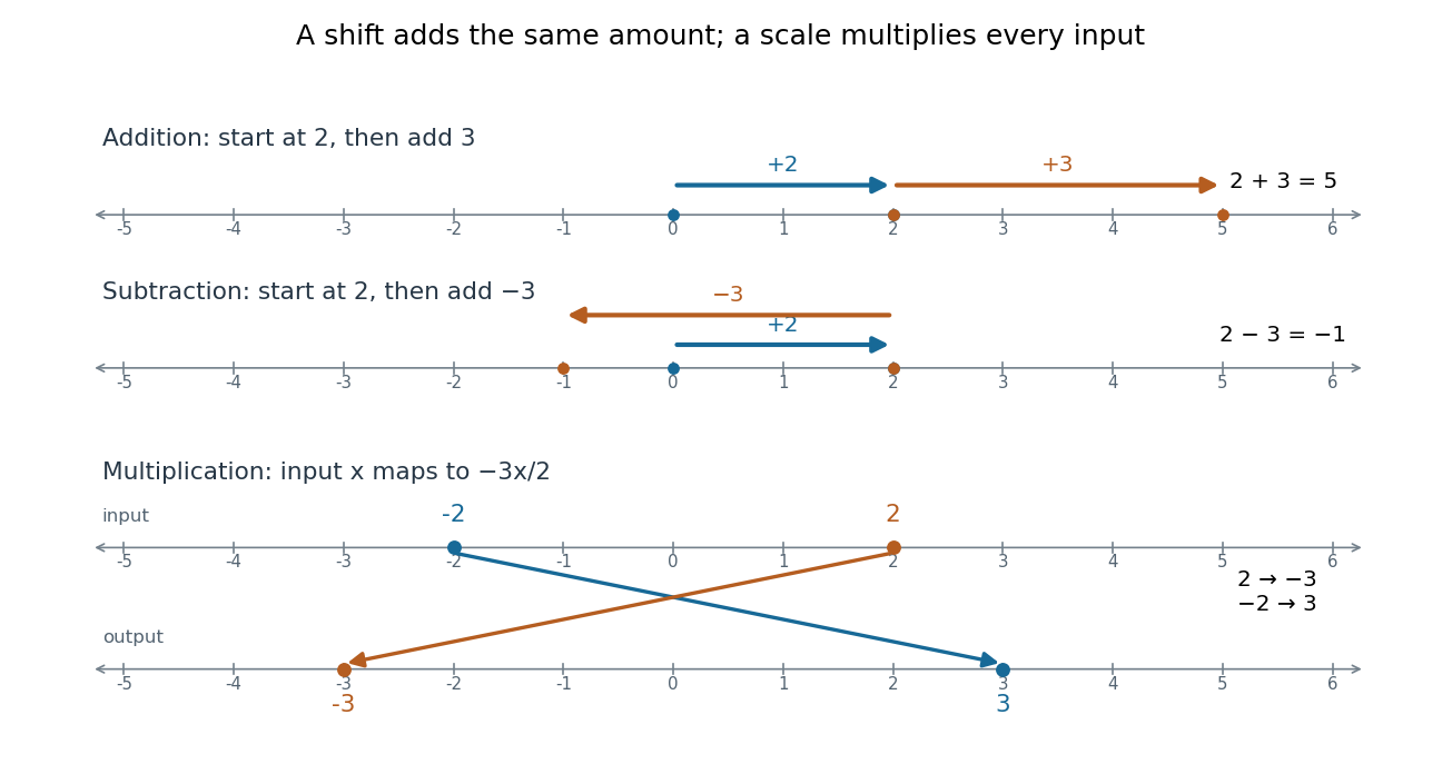
Addition shifts positions on a number line, while a negative multiplication factor changes both scale and direction
. **Details**.

The bottom panel applies

x \mapsto - 3 x /2

. Input

2

becomes

- 3

, and input

- 2

becomes

3

. Multiplication by a negative real number rescales distances from zero and reverses direction, giving a reflection in mathematics as well as a scale change. This is a different operation from shifting every input by one fixed amount.

 Read the full article

Addition chain 2026-10-20

 View more

An addition chain for a positive integer

k

1 = a_{0} < a_{1} < \dots < a_{r} = k

, where each

a_{t}

is the sum of two earlier entries, which may coincide. It computes

x^{k}

r

multiplications by reusing previously computed powers. For example,

1, 2, 3, 6, 12, 15

computes

x^{15}

in five multiplications.

 Read the full article

Arbitrary-precision arithmetic 2026-10-20

 View more

Integer arithmetic in which storage grows with the number of numerical digits needed, instead of imposing a fixed word size. It allows exact addition, multiplication, and exponentiation on large integers, subject to available memory; operation costs grow with operand length.

 Read the full article

Arithmetic Created 2026-09-24 Updated 2026-10-13

 View more

Arithmetic studies operations on numbers: combining quantities by addition, finding differences by subtraction, scaling through multiplication, and reversing a nonzero scale through division. Its usefulness goes beyond producing an answer. A calculation can express how resources are shared, how a measurement changes with scale, or why two different descriptions of a quantity agree.

The allowed numbers matter. Start with the natural numbers

0, 1, 2, \dots

. Counting collections gives

2 + 3 = 5

, but removing three from two calls for the integer

- 1

. Sharing three units equally between two recipients gives the rational number

3/2

. These operations motivate larger number systems: integers supply additive inverses, and rational numbers supply division by nonzero integers. A real number can also express lengths such as a diagonal of Euclidean norm

2

, which is not a rational number.

The beauty is that bookkeeping, geometry, and algebra can check one another. The same product

3 (2 + 4) = 18

counts three groups of six, measures the area of a rectangle, and splits as

3 \cdot 2 + 3 \cdot 4

by distributivity. A number line makes negative integers visible as positions; a fraction records an exact share even when its decimal representation does not terminate. An arithmetic rule becomes easier to remember when these interpretations fit together.

 Read the full article

Arithmetic circuit 2026-10-18

 View more

An arithmetic circuit is a Directed acyclic graph whose input nodes are variables or constants in a field, and whose internal gates perform addition, subtraction, or multiplication. Gates may reuse earlier outputs, so the circuit can represent a polynomial without listing all its monomials.

 Read the full article

Binary powering multiplication count Created 2026-10-14 Updated 2026-10-24

 View more

For the optimized left-to-right exponentiation by squaring algorithm, let

ℓ = ⌊ lo g_{2} n ⌋ + 1

be the length of the binary expansion of a positive integer

n

, and let

w = wt (n)

be its Hamming weight, the number of digits equal to one. There are exactly

ℓ - 1

digits after the leading one, and exactly

w - 1

remaining ones. Therefore the count is

S (n) = ℓ - 1, T (n) = w - 1, C (n) = S (n) + T (n) = ℓ + w - 2.

(1)

Here

S

counts squarings and

T

counts further multiplications by the base; every squaring counts as one multiplication in $C$ . Assignment, digit reading, and any inversion are outside this count. The formula includes

n = 1

, which requires zero multiplications; define

C (0) = 0

separately.

For a fixed length

ℓ

, the bounds are

ℓ - 1 \leq C (n) \leq 2 ℓ - 2

. A power of two reaches the lower bound because its Hamming weight is one;

n = 2^{ℓ} - 1

reaches the upper bound because all digits are one. For

n = 13

ℓ = 4

and

w = 3

, giving

C (13) = 5

. Thus the arithmetic operation count is

O (lo g (n + 1))

in Big O notation, but inputs of similar magnitude can have different counts.

Figure 1.
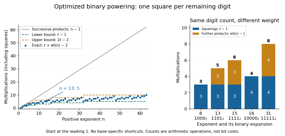
Exact multiplication counts for optimized exponentiation by squaring depend on binary length and Hamming weight
. For positive exponents through $63$ , dots show $C (n) = ℓ + wt (n) - 2$ , including each squaring. The dashed curves bound all counts at each binary length. Successive multiplication needs $n - 1$ operations. The second panel compares squarings and further multiplications for exponents $8, 13, 15, 16, 31$ . These are exact counts, not timing measurements. **Details**.

This is a count for the specified algorithm, not a claim that it always minimizes multiplications among all methods. For instance, at

n = 15

the count is six, but the powers with exponents

1, 2, 3, 6, 12, 15

can be built in five multiplications: square, multiply by

a

, square, square, then multiply by the already stored

a^{3}

. Saving operations this way uses a different schedule and stored intermediate powers.

 Read the full article

Bit cost of modular exponentiation 2026-10-14

 View more

The binary powering multiplication count counts arithmetic operations. The time complexity measured in operations on individual bits also depends on operand lengths. Put

L = ⌊ lo g_{2} m ⌋ + 1

, the binary length of the modulus, and let

ℓ

be the positive exponent's binary length. Stored residues use at most

L

bits, and an unreduced product uses at most

2 L

bits.

With ordinary long multiplication and division with remainder, one modular product costs

O (L^{2})

operations on bits. Combining that cost with

O (ℓ)

modular products gives

bit cost of the powering loop = O (ℓ L^{2}) .

(1)

This bound includes reductions in the loop, and assumes the base has already been reduced and the exponent is available as a binary expansion. Reading the exponent takes

O (ℓ)

additional work; initial reduction of a very long base depends on its input length, and an inverse for a negative exponent adds further work. More generally, if a modular product costs

R (L)

operations on bits, the powering loop costs

O (ℓ R (L))

. Faster multiplication and reduction methods can improve the quadratic bound.^[ref]

For ordinary integer powers with

∣ a ∣ \geq 2

, the output itself has

⌊ n lo g_{2} ∣ a ∣ ⌋ + 1

binary digits. Even writing it takes work proportional to that length. Consequently

O (lo g (n + 1))

multiplications does not imply

O (lo g (n + 1))

operations on bits: the operands grow during ordinary exponentiation by squaring, whereas modular exponentiation keeps them bounded by the modulus. A squaring or multiplication by a small fixed base can also cost less than a general product, so equal counts need not mean equal running times.

 Read the full article

Boolean matrix multiplication 2026-10-31

 View more

For Boolean matrices, replace numerical addition by logical disjunction and multiplication by logical conjunction. Applied to adjacency matrices, the product records a walk formed by following one segment represented by the first matrix and one represented by the second. For an adjacency matrix

A

n \geq 1

vertices, start from

I \lor A

. Repeated squaring then computes reflexive transitive closure once the exponent reaches

n - 1

: the identity entries pad shorter walks, and every reachable pair has a simple path of length at most

n - 1

 Read the full article

Chinese remainder theorem Created 2026-09-24 Updated 2026-10-20

 View more

The Chinese remainder theorem says that remainders modulo pairwise coprime positive integers can be specified independently. For

m_{1}, \dots, m_{r}

pairwise coprime and

M = m_{1} \dots m_{r}

, every prescribed list

a_{1}, \dots, a_{r}

determines one congruence class modulo $M$ satisfying

x \equiv a_{j} (mod m_{j})

for all

j

. It determines a class, rather than one unrestricted integer: adding a multiple of

M

preserves every remainder.

For example, combine

x \equiv 2 (mod 3)

and

x \equiv 3 (mod 5)

. Write

x = 2 + 3 k

from the first condition. The second becomes

3 k \equiv 1 (mod 5)

. Since three has modular inverse two modulo five,

k \equiv 2 (mod 5)

, giving $x \equiv 8 (mod 15)$ . The integers

8

23

and

- 7

all work. The fifteen possibilities modulo fifteen correspond to the fifteen pairs in a three-by-five grid.

Figure 1.
Coprime moduli fill every residue pair; shared factors impose a compatibility condition
. **Details**.

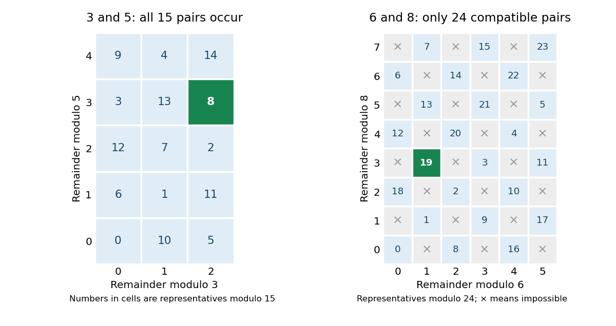
The theorem also preserves arithmetic: reducing an addition or a multiplication modulo each

m_{j}

gives the same tuple as performing that operation on the corresponding congruence classes. In the language of quotient rings, reduction is a ring isomorphism

Z / M Z [x]_{M} ⟶ j = 1 \prod r Z / m_{j} Z, ⟼ ([x]_{m_{1}}, \dots, [x]_{m_{r}}) .

(1)

One large residue is thus an exact encoding of several smaller residues. This is useful for splitting arithmetic into smaller calculations and then reconstructing the result; MIT's modular arithmetic notes develop both the reconstruction and the product representation. ^[ref] For a concrete multiplication,

7

corresponds to

(1, 2)

and

8

(2, 3)

modulo

(3, 5)

. Their componentwise product is

(2, 1)

, which reconstructs to

11 (mod 15)

, agreeing with

56 \equiv 11 (mod 15)

A constructive formula explains the independence. For

m_{j} > 1

, put

M_{j} = M / m_{j}

and choose

u_{j}

with

M_{j} u_{j} \equiv 1 (mod m_{j})

, using a modular multiplicative inverse. Then

e_{j} = M_{j} u_{j}

is one modulo

m_{j}

and zero modulo every other

m_{i}

. Therefore

x \equiv \sum_{j = 1}^{r} a_{j} e_{j} (mod M)

(2)

has the desired remainders. A modulus equal to one imposes no restriction and can be omitted. Uniqueness follows because a difference divisible by every

m_{j}

is divisible by their product when they are pairwise coprime. This short construction gives a reusable algorithm as well as an existence statement.

The coprime hypothesis explains why every cell in the left grid is attainable. With integer moduli six and eight, a pair must agree modulo their greatest common divisor, two. There are twenty-four compatible pairs, rather than forty-eight arbitrary pairs; each corresponds to a class modulo the least common multiple, twenty-four. The Chinese remainder theorem for noncoprime moduli states the resulting compatibility rule.

 Read the full article

Commutative ring Created 2026-09-24 Updated 2026-10-14

 View more

A commutative ring is a ring in which multiplication satisfies

ab = ba

for every pair. The integers and the polynomial ring

Z [X]

are examples. So is

Z / n Z

, the quotient ring whose elements are residue classes in modular arithmetic. We represent these by

0, 1, \dots, n - 1

and reduce each sum or product to its remainder. All following calculations modulo

6

use this convention.

Z /6 Z

2 \cdot 3 = 0

, although neither factor is zero. Thus

2

and

3

are zero divisors: nonzero elements whose product with another nonzero element can vanish. Also

2 \cdot 1 = 2 \cdot 4 = 2

. Removing the common factor

2

would falsely assert

1 = 4

. The entire row for multiplication by

2

2 \cdot (0, 1, 2, 3, 4, 5) = (0, 2, 4, 0, 2, 4) .

(1)

The repetitions explain the linear congruences directly. The equation

2 x = 2

has exactly the two solutions

x = 1, 4

, whereas

2 x = 1

has none. A common factor can erase information, and a nonzero coefficient does not guarantee that an equation has a solution.

Figure 1.
Multiplication modulo 6 repeats outputs, while every nonzero row modulo 5 is a permutation
. **Details**.

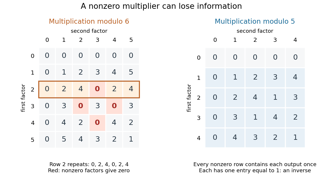
A unit in a ring is an element

u

with a multiplicative inverse, meaning

uv = vu = 1

for some

v

. In

Z /6 Z

, the units are exactly

1

and

5

, since

5^{2} = 1

. The other nonzero elements,

2, 3, 4

, are zero divisors; for

4

, use

4 \cdot 3 = 0

. In a nonzero commutative ring, a unit cannot be a zero divisor: multiplying

u b = 0

by its multiplicative inverse forces

b = 0

. But a nonzero element need not be a unit or a zero divisor: the integer

2

is neither in

Z

By contrast, in

Z /5 Z

, every row for a nonzero multiplier is a permutation of

0, 1, 2, 3, 4

. Each such row contains

1

exactly once, giving a multiplicative inverse:

1^{- 1} = 1

2^{- 1} = 3

3^{- 1} = 2

, and

4^{- 1} = 4

. Hence this commutative ring is a field. For example,

2 x = 1

now has the unique solution

x = 3

. Reading the tables reveals which algebraic steps the arithmetic permits.

 Read the full article

Compilation arithmetic example 2026-10-14

 View more

Consider the program expression x*(2+3)-4 in a deliberately small programming language. Its only program identifier is x, supplied as an integer input. Its literal values are nonnegative decimal numerals, interpreted as integers. Whitespace is ignored between lexical tokens. Its context-free grammar is:

expression ::= term (("+" | "-") term)*
term       ::= factor ("*" factor)*
factor     ::= numeral | "x" | "(" expression ")"
numeral    ::= digit digit*
digit      ::= "0" | "1" | "2" | "3" | "4"
             | "5" | "6" | "7" | "8" | "9"

Here * outside quotation marks means zero or more repetitions. Repeated operators are grouped to the left, specifying operator associativity; term gives multiplication higher operator precedence than addition and subtraction. Parentheses override that grouping. There is no unary minus, variable assignment, function call, or side effect in this language. Evaluation obtains each left operand before its right operand and uses exact integer arithmetic, with no fixed-width overflow.

Lexical analysis recognizes x, *, (, 2, +, 3, ), -, 4. Parsing constructs the concrete abstract syntax tree Sub(Mul(Name(x), Add(Int(2), Int(3))), Int(4)). Parentheses have done their work by making Add a child of Mul; they need not survive as nodes. Constant folding changes this to Sub(Mul(Name(x), Int(5)), Int(4)). It cannot replace Name(x) by a literal value because the input is supplied at execution. The resulting function of the input is

f (x) = 5 x - 4

A compiler for our stack machine emits LOAD x; PUSH 5; MUL; PUSH 4; SUB. LOAD x pushes the current input; PUSH n pushes the integer literal value n. Each binary instruction removes the top item as its right operand, then the next item as its left operand, and pushes the result. The instruction sequence is an intermediate representation that an interpreter can execute; no machine code has been emitted. A compact binary encoding could make it bytecode, but these printed instruction names are only a readable notation.

Why does this compilation preserve the result? A structural induction supplies a short proof outline. Translating a literal value or x appends its value to any initial stack. For a binary abstract syntax tree node, first translating the left child and then the right child appends the two operand values; the matching instruction replaces them by exactly the original operation's result. Previously present stack items remain intact. Constant folding also preserves the result because

2 + 3 = 5

in the specified integer arithmetic. Together these facts explain agreement for every integer input, rather than merely agreement for one trial.

 Read the full article

Complex number Created 2026-09-24 Updated 2026-10-14

 View more

A complex number is

z = x + i y

, where

x, y

are real numbers and the imaginary unit satisfies

i^{2} = - 1

. The real part is

x

and the imaginary part is

y

: for

3 + 4 i

they are

3

and

4

, respectively. Equality requires both coordinates to agree. Thus the complex plane gives each complex number a concrete position, while ordinary addition and multiplication become geometric operations.

For

z = 3 + 4 i

and

w = 1 + i

, addition works coordinate by coordinate, whereas multiplication uses

i^{2} = - 1

z + w = 4 + 5 i, z w = (3 + 4 i) (1 + i) = 3 + 7 i - 4 = - 1 + 7 i .

(1)

These answers encode different motions: addition by

w

is a translation, while multiplication by

w

is a rotation combined with a uniform change of size. Keeping these pictures distinct prevents a common beginner's confusion.

The complex numbers form a field: every nonzero

z

has a multiplicative inverse, computable using its complex conjugate and modulus. They also supply the missing solutions of a quadratic equation such as

u^{2} + 1 = 0

, namely

u = \pm i

. The surprising payoff is that extending arithmetic also makes Euclidean geometry easier to calculate. For a systematic introduction to these definitions, see Jeremy Orloff, MIT 18.04, topic 1, sections 1.3–1.5.

 Read the full article

Complex plane Created 2026-09-24 Updated 2026-10-14

 View more

The complex plane identifies the complex number

x + i y

with the point

(x, y)

in Cartesian coordinates. The horizontal coordinate is its real part, the vertical coordinate its imaginary part. Arrows from zero identify the same points with vectors. Adding

1 + i

moves

3 + 4 i

4 + 5 i

: every point undergoes the same translation.

Multiplication has a richer geometry. Multiplying by the imaginary unit sends

x + i y

- y + i x

, a counterclockwise quarter-turn rotation. In particular

i (3 + 4 i) = - 4 + 3 i

. Multiplying by

1 + i

rotates through

π /4

and scales every Euclidean distance by

2

. More generally, multiplication by

a + ib

acts through the real matrix

(x y) ⟼ (a b - b a) (x y) .

(1)

For

a + ib \neq = 0

, this preserves oriented angles between nonzero displacement vectors: every direction turns equally. Its determinant is

a^{2} + b^{2} > 0

, while its common scale is

a^{2} + b^{2}

. This is the elementary geometric reason complex numbers are so useful for conformal maps.

The name Argand plane recalls Jean-Robert Argand's geometric interpretation. In his 1813 article he explicitly reports publishing his Essai in 1806; the original article is available in Argand, Annales de mathématiques, volume 4, page 133. A ^[ref] preserves the essay and its geometric drawings. Reading these alongside a modern complex plane reveals how directions and lengths give arithmetic a visible meaning.

 Read the full article

Congruence modulo an ideal 2026-10-14

 View more

Two elements of a commutative ring are congruent modulo an ideal if their difference lies in that ideal, equivalently if their images in the quotient ring agree. This is an equivalence relation compatible with addition and multiplication. For

R = Z_{p} [[T]]

and

I = p^{k} R

, it means every coefficient difference is divisible by

p^{k}

 Read the full article

Constant folding 2026-10-13

 View more

Constant folding replaces a program expression whose value is known during translation by a literal value. For x=2+3*4, first replace the multiplication subtree by Constant(value=12), then replace the addition subtree by Constant(value=14). The variable assignment and its Store target survive: the result still assigns to x. This illustrates why a bottom-up abstract syntax tree traversal is convenient: replacing one child can make its parent eligible for the next replacement.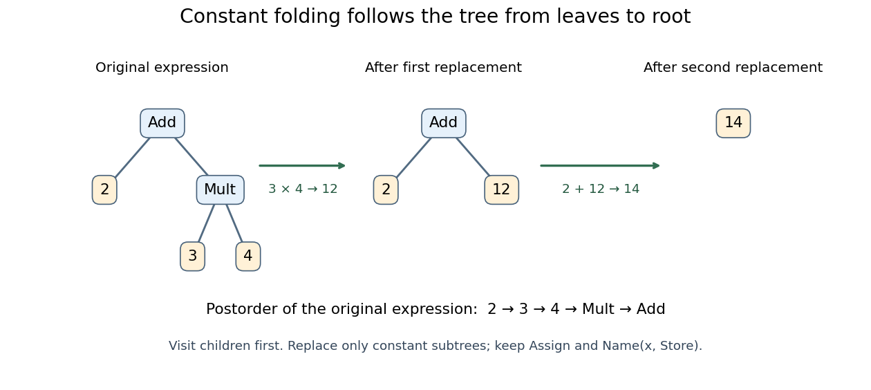

Figure 1.
Constant folding and postorder abstract syntax tree traversal for `2+3*4`: replace $3 \cdot 4$ by $12$ , then $2 + 12$ by $14$
. **Details**.

Here is a deliberately small Python transformer. Calling generic_visit first transforms the children; returning a node replaces the visited node. The location helpers retain or supply the metadata expected for compilation. ^[ref]

class FoldIntegers(ast.NodeTransformer):
    def visit_BinOp(self, node):
        self.generic_visit(node)
        if (isinstance(node.left, ast.Constant)
                and isinstance(node.right, ast.Constant)
                and type(node.left.value) is int
                and type(node.right.value) is int
                and type(node.op) in OPS):
            value = OPS[type(node.op)](node.left.value, node.right.value)
            return ast.copy_location(ast.Constant(value=value), node)
        return node

tree = ast.parse("x=2+3*4", optimize=0)
folded = ast.fix_missing_locations(FoldIntegers().visit(tree))
namespace = {}
exec(compile(folded, "<folded example>", "exec"), namespace)
assert namespace["x"] == 14
assert ast.unparse(folded) == "x = 14"

This transformer folds literal integer operands only. It leaves a+3*4 as a+12, without inventing a value for the program identifier a. It leaves calls intact: replacing 0*f() by 0 could discard a side effect or a failure. Nor does it reassociate floating-point arithmetic, where changing parentheses can change rounding. For the supported integer arithmetic, a short structural induction explains correctness: a retained literal value has the same value; at each folded binary node, the already-correct child values are combined by exactly the original operation in the original left/right order. This claim concerns the supported fragment's values, not unrestricted equivalence of arbitrary Python programs.

 Read the full article

Continuous function Created 2026-09-24 Updated 2026-10-14

 View more

A continuous function sends sufficiently nearby function inputs to nearby function outputs. For a real-valued function

f : D \to R

and a point

a \in D

that is an accumulation point of

D

, this means

lim_{x \to a x \in D} f (x) = f (a) .

(1)

The approached value and the assigned value must agree. Continuity on

D

means continuity at every point of the domain of a function. At an endpoint of an interval, only approaches inside that domain of a function count. The epsilon-delta definition of continuity below also applies at an isolated point, where continuity holds automatically.^[ref]

For the polynomial function

f (x) = x^{2}

, approaching

1

makes the function output approach

f (1) = 1

. The continuity bounds for the square function turn this observation into an explicit guarantee:

∣ x - 1∣ < 0.2

implies

∣ x^{2} - 1∣ < 0.6

. This is useful whenever a small error in an function input must produce a controlled error in an function output. The required input tolerance can depend on the point and on the chosen output tolerance.

The absolute value function

g (x) = ∣ x ∣

is also a continuous function, including at zero:

∣ g (x) - g (0) ∣ = ∣ x ∣

. But its left and right derivatives there are

- 1

and

1

, so it is not a differentiable function at zero. Continuity controls values without requiring a tangent line. Conversely, a differentiable function is continuous wherever it is differentiable: if

f (a + h) - f (a) = h (f^{'} (a) + o (1))

, the difference tends to zero with

h

Several useful consequences reuse this one local idea. Addition, multiplication and function composition preserve continuity; a quotient of functions is continuous where its denominator is nonzero. On an interval, the intermediate value theorem turns continuity into a guarantee that no intermediate function output is skipped. On a compact set, the extreme value theorem guarantees attained maximum and minimum values. Those extra hypotheses matter: continuity alone on an unbounded domain of a function does not provide a global bound or an attained global maximum.

A rational function such as

x \mapsto 1/ x

is continuous on its domain of a function

R ∖ {0}

. Zero is excluded from that domain of a function; the missing point prevents a continuous extension there, but it does not make the existing map discontinuous at one of its actual inputs. Always state the domain of a function before judging continuity.

 Read the full article

Correct operations through an abstraction function 2026-10-14

 View more

For a deterministic binary operation on an abstract data type, let

f

be its specified operation on abstract values and

F

the implementation on concrete states. For every permitted valid input pair

(r, s)

, require both

I (F (r, s)) and α (F (r, s)) = f (α (r), α (s)) .

(1)

The first condition preserves the representation invariant. The second makes a commutative diagram: either execute

F

and then apply the abstraction function, or apply the abstraction function to both inputs and then execute the abstract operation

f

; both paths reach the same value. These conditions state functional correctness of a completed operation; termination is an additional obligation for algorithm correctness.^[ref]

For addition in the unreduced rational representation, choose

f (x, y) = x + y, F ((a, b), (c, d)) = (a d + b c, b d) .

(2)

For example,

F ((1, 2), (1, 3)) = (5, 6)

represents

5/6

, precisely the sum of

1/2

and

1/3

. The short correctness argument uses nonzero denominators:

b \neq = 0

and

d \neq = 0

imply

b d \neq = 0

, preserving the representation invariant, and

α (F ((a, b), (c, d))) = \frac{a d + b c}{b d} = \frac{a}{b} + \frac{c}{d} = f (α (a, b), α (c, d)) .

(3)

Figure 1.
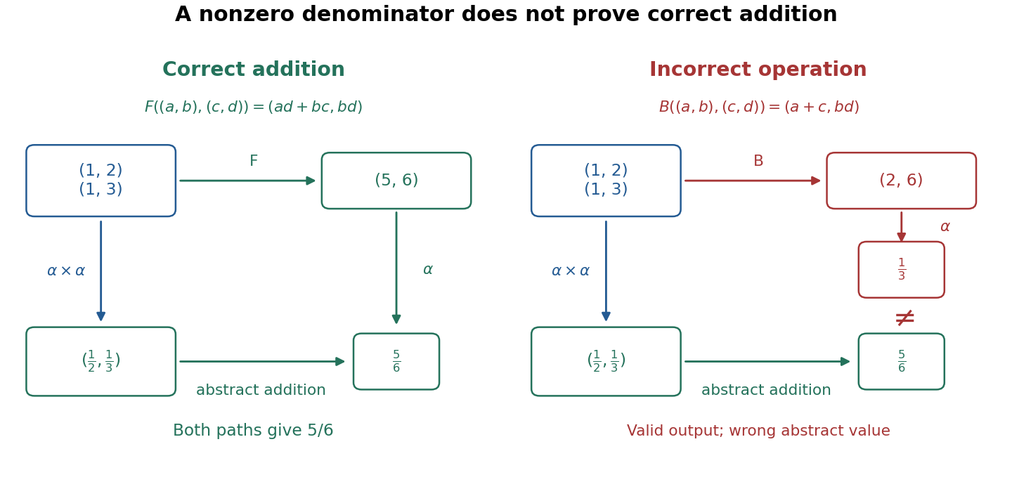
Correct rational addition makes both paths agree; an invariant-preserving incorrect operation gives a different value
. **Details**.

Now consider an incorrect implementation that uses addition on the numerators and multiplication on the denominators:

B ((a, b), (c, d)) = (a + c, b d) .

(4)

It preserves the representation invariant for every valid input pair because its denominator is still

b d \neq = 0

. Yet

B ((1, 2), (1, 3)) = (2, 6)

represents

1/3

, not the specified sum

5/6

. Even perfect checks of the representation invariant before and after this call would miss the error: the result is a legal representation of the wrong rational number.

The incorrect operation also exposes an accidental dependence on representation. Replace

(1, 2)

by the equivalent state

(2, 4)

while keeping

(1, 3)

. The correct operation gives

(10, 12)

, still representing

5/6

; the incorrect operation gives

(3, 12)

, representing

1/4

instead of its previous

1/3

. A correct addition must yield the same abstract result for equivalent inputs, although its concrete outputs may differ. This is why checks against the formal specification should compare abstract values, including unreduced representations and representations with a negative denominator, rather than demand identical stored pairs.

The calculation assumes exact integers. An implementation with bounded storage must additionally specify how it handles products and sums outside its supported range; the mathematical argument alone does not establish its functional correctness. The bounded queue with encapsulation illustrates the corresponding need to account for returned status values and failed operations, alongside the abstract state transition.

 Read the full article

Coupled binary exponentiation 2026-10-31

 View more

To compute two nonnegative integer powers in one while loop, maintain a separate accumulator, current base and remaining exponent for each exponentiation by squaring. The paired loop invariant is

p x^{k} = A^{n}

and

q y^{l} = B^{m}

. For each positive remaining exponent, transfer its odd factor to its accumulator and halve the exponent while squaring its base. A zero remaining exponent is left unchanged. The mathematical integer

k + l

is a loop variant: at least one positive term strictly decreases in every iteration. Both powers are therefore complete when the loop stops. The iteration count is

O (lo g (max (n, m) + 1))

, with constant space and a constant number of multiplications per iteration. This is an exact-arithmetic identity; floating-point rounding introduces a separate error in a numerical implementation.

 Read the full article