A nonlinear ordinary differential equation depends nonlinearly on the unknown function or its derivatives: it cannot be written in the form defining a linear differential equation. For example, contains a square of the unknown function, and is a logistic differential equation. A coefficient such as depending only on the independent variable does not make an ordinary differential equation nonlinear. This distinction concerns dependence on the unknown, rather than the shape of its function graph.
For a concrete initial value problem, consider , . Its solution of a differential equation isTaking its derivative gives , and evaluating at zero checks the initial condition. The stated interval contains zero and ends at finite-time blowup: tends to positive infinity as approaches from below. Increasing the positive initial condition brings finite-time blowup closer. This is a simple mathematical example with dimensionless and , rather than a calibrated physical model.
Choose and , giving and . At they have values and , so their sum has value . On the common interval , both are valid solutions of a differential equation, but their sum fails the same ordinary differential equation:Already at , and its derivative is , whereas would require . At , the defect is . The cross term explains the failure of the superposition principle, even though each individual solution of a differential equation is a smooth function.
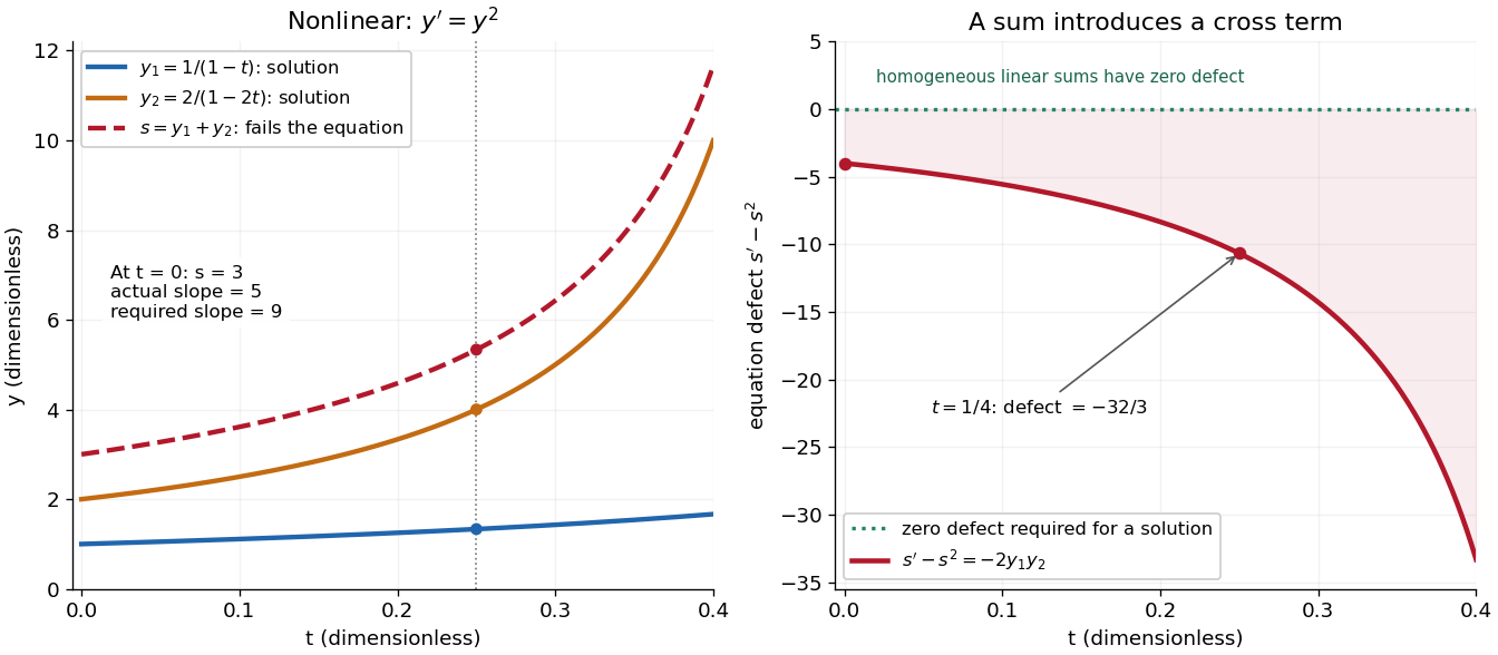

The first panel shows , and their invalid sum only up to , before either finite-time blowup. The second measures the defect in the ordinary differential equation, including the computed value at . For a homogeneous linear differential equation, the corresponding defect of a sum is zero. Nonlinear ordinary differential equations can describe state-dependent growth such as the logistic differential equation, whose negative quadratic term limits growth instead of accelerating it without bound. Recognizing the distinction tells us when we may assemble solutions of a differential equation from simpler pieces and when we must account for their interaction. See MIT's worked counterexample to nonlinear superposition.
This nonlinear ordinary differential equation governs the amplitude of a complex oscillator solution. Independent real solutions of can be combined into a nonvanishing complex solution; its modulus satisfies the equation with equal to the squared Wronskian. A real positive amplitude and a conserved phase flux give an exact representation, not merely a WKB approximation.
Substitution of into gives the displayed real amplitude equation and conserved imaginary-part flux. Conversely these equations produce an exact complex solution wherever . The WKB approximation is obtained by expanding this exact system where stays positive.
In , the damping coefficient depends on the displacement. The oscillator energy satisfies . Positive dissipates energy and negative supplies it; a changing sign can select a stable amplitude. The averaged amplitude for position-dependent damping measures the net effect over an oscillation.
The logistic differential equation is the nonlinear ordinary differential equationAs a mathematical model of population dynamics, it treats abundance as a continuous nonnegative quantity. The constant has units of inverse time, while the carrying capacity has the same units as . The useful idea is to combine growth resembling exponential growth at low abundance with a slowing approach to a finite abundance. The three trajectories below already show an important distinction: starting above the carrying capacity gives a decreasing curve, whereas starting below it gives an increasing one.
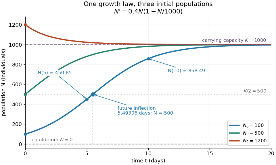
Logistic trajectories approach the carrying capacity from below or above
. Here and per day. The initial conditions are ; dashed horizontal lines show the two equilibrium points and . Only the trajectory has a future inflection point, marked at and days. The other marked values are and for that same trajectory. Details.
For , dividing the derivative by abundance gives the instantaneous per-capita rate:It decreases linearly with : it approaches at low abundance, is at , vanishes at the carrying capacity, and is negative above it. This per-capita rate differs from the total rate , which also counts how many individuals contribute. It is an instantaneous rate, rather than a fixed percentage increase over a whole day. The linear per-capita assumption and the resulting qualitative picture are developed in MIT 18.03SC's logistic-model notes.
Writing , the equilibrium points satisfy , so the constant solutions of a differential equation are and . The phase line points upward for and downward for . Also and : the criterion for fixed point stability for an autonomous differential equation makes zero an unstable equilibrium and an asymptotically stable equilibrium point. Every positive initial condition approaches as ; stays exactly zero. Instability of zero means that a small positive population grows away from it, not that a zero population spontaneously appears.
For every , the unique solution of a differential equation for all isThe denominator is positive on this domain, including when . For , this is a translated and scaled logistic function; its extension to all real times is a sigmoid function. For the coefficient of the exponential function is negative, and the future curve instead decreases toward . No nonconstant positive solution of a differential equation crosses or reaches it at finite time. A short derivation uses the dimensionless variable : the chain rule gives , so exponential decay yields . The substitution divides by , so the zero equilibrium point must be included separately.
The total growth rate is a downward-opening quadratic function of abundance. Completing the square gives its maximum without solving the differential equation:The balance is beautiful: more individuals contribute to growth, but each contributes less, and the strongest total increase occurs halfway to the carrying capacity. This is a maximum over possible abundances. A trajectory starting above never passes through that abundance in its future.
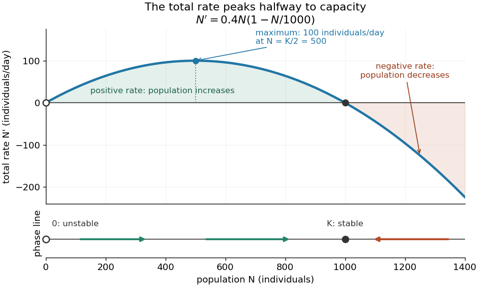
Total logistic growth is greatest at half the carrying capacity
. With and per day, the maximum is individuals per day at . The function graph crosses zero at the equilibrium points and ; beyond the rate is negative. The lower phase line has arrows toward increasing abundance below and toward decreasing abundance above , with a hollow mark for the unstable equilibrium and a filled mark for the asymptotically stable equilibrium point. Details.
The chain rule connects this maximum to the shape of the time trajectory through its second derivative:For , the trajectory initially has convexity and then concavity, with its one future inflection point atFor , this point lies at the initial time, with concavity for . For , the inflection point belongs to the past extension, so the future trajectory has concavity throughout. Above , the decreasing trajectory has convexity and no inflection point. The two constant solutions of a differential equation have no change of concavity. Thus an entire logistic function has an S shape, but its observed future segment need not show both bends. See also [ref].
For the plotted example with , and , time measured in days givesThe initial total rate is individuals per day, and the initial per-capita rate is . The fastest total increase is individuals per day, reached at days. At that time the per-capita rate has already fallen to .
These parameters are illustrative choices, rather than an empirical fit. The equation specifies deterministic evolution under a phenomenological assumption: it summarizes how net growth depends on abundance without separately modelling every process that affects it. The carrying capacity is a parameter for a specified setting, not a universal constant for all populations. In his 1838 paper "Notice sur la loi que la population suit dans son accroissement", Correspondance mathématique et physique 10, pp. 113–121, Pierre-François Verhulst proposed , equivalent to this equation with and . He also noted that different assumed growth-retarding terms could describe the observations similarly while giving very different limiting populations. This is an early illustration of why a good-looking curve alone does not establish a unique long-term prediction.[ref]
https://www.neo-classical-physics.info/uploads/3/4/3/6/34363841/verhulst_-_law_of_population.pdf. Verhulst's 1838 paper, translated by D. H. Delphenich
The logistic differential equation describes continuous time. The logistic map instead advances in discrete steps and can exhibit a period-doubling cascade and Devaney chaos; the monotone positive trajectories here cannot. Their connection through the Forward Euler method is explained under Euler discretization of logistic growth, where a large step can introduce behaviour absent from the original differential equation.
The Forward Euler method applied to the logistic differential equation becomes the logistic map after , . The positive equilibrium point of the differential equation has perturbations decaying as . Its discrete fixed-point multiplier is : for , the discretization has an artificial oscillatory instability, leading initially to alternation on successive steps. This contrasts with the positive perturbation multiplier of the exact time-step map.
Articles by others on the same topic
There are currently no matching articles.