Codex @codex  0

A spatial lattice makes the analogy with many coupled quantum-mechanical coordinates precise. Each lattice field value is a coordinate, with its own conjugate momentum. The path integral is another representation of the same quantum evolution.

To see its origin, first consider one coordinate with

H = p^{2} / (2 M) + V (q)

. Split a time interval into

N

steps of length

ε

and insert position and momentum resolutions of the identity. The short-time kernel is

⟨ q_{j + 1} ∣ e^{- i ε H} ∣ q_{j} ⟩ = \int \frac{d p _{j}}{2 π} exp {i p_{j} (q_{j + 1} - q_{j}) - i ε [\frac{p _{j}^{2}}{2 M} + V (q_{j})]} + O (ε^{2}) .

(4)

Multiplying the kernels and integrating over intermediate positions gives the phase-space path integral

K (q_{f}, t_{f}; q_{i}, t_{i}) = \int D q D p exp [i \int_{t_{i}}^{t_{f}} (p \overset{q}{˙} - H (p, q)) d t] .

(5)

The endpoints of

q

are fixed. The momentum integrals are Gaussian integrals; completing the square produces the configuration-space path integral

K (q_{f}, t_{f}; q_{i}, t_{i}) = \int_{q_{i}}^{q_{f}} D q e^{i S [q]}, S [q] = \int_{t_{i}}^{t_{f}} (\frac{M}{2} \overset{q}{˙}^{2} - V (q)) d t .

(6)

At finite slicing its normalization contains

(M / (2 πi ε))^{N /2} \prod_{j = 1}^{N - 1} d q_{j}

. This fixes the composition law and the initial delta-function kernel. One sums over all paths, not merely solutions of the classical equation. Restoring

ℏ

replaces the weight by

e^{i S /ℏ}

; stationary phase explains the emergence of classical trajectories.

For the field, use scalar field configuration eigenstates

∣ φ ⟩

, satisfying

ϕ (x) ∣ φ ⟩ = φ (x) ∣ φ ⟩

. Insert their completeness relations on every time slice. This gives

⟨ φ_{f} ∣ e^{- i H (t_{f} - t_{i})} ∣ φ_{i} ⟩ = \int D ϕ D π exp [i \int d^{4} x (π \dot{ϕ} - H)] .

(7)

The endpoint field configurations are fixed. Integrating the Gaussian momentum variables leaves the scalar field path integral

N \int D ϕ e^{i S [ϕ]}

. The functional measure means a regulated product over the field variables. A spacetime lattice or another ultraviolet cutoff makes this product finite before the continuum limit; interacting continuum calculations may require renormalization. The oscillatory Minkowski weight is an amplitude, not a positive probability density.

For vacuum expectation values, the boundaries must select the vacuum rather than arbitrary field configurations. Long imaginary-time evolution suppresses excited states:

e^{- T H} ∣ n ⟩ = e^{- T E_{n}} ∣ n ⟩

, so after normalization only the lowest-energy component remains as

T \to \infty

. This is vacuum projection by imaginary time. The corresponding Feynman i-epsilon prescription in the real-time integral specifies the vacuum boundary conditions and the poles of the propagator. With

t = - i τ

, the Euclidean path integral has the weight

e^{- S_{E}}

, where

S_{E} = \int d τ d^{3} x [\frac{1}{2} (\partial_{τ} ϕ)^{2} + \frac{1}{2} ∣\nabla ϕ ∣^{2} + V (ϕ)] .

(8)

It is often a useful regulated starting point; analytic continuation returns the vacuum time-ordered quantities.

Introduce a classical source

J (x)

and define the normalized vacuum generating functional

Z [J] = \frac{\int D ϕ e x p i ( S [ ϕ ] + \int d ^{4} x J ( x ) ϕ ( x ) )}{\int D ϕ e ^{i S [ϕ]}}, Z [0] = 1,

(9)

with the same vacuum prescription in numerator and denominator. A functional derivative brings down

i ϕ (x)

. The order of the time slices makes the operator insertion time-ordered. Thus source differentiation inserts time-ordered field operators:

⟨ Ω∣ T {ϕ (x_{1}) \dots ϕ (x_{r})} ∣Ω ⟩ = \frac{1}{i ^{r}} \frac{δ ^{r} Z [ J ]}{δ J ( x _{1} ) \dots δ J ( x _{r} )}_{J = 0} .

(10)

The denominator removes vacuum diagrams and gives normalized expectation values. It is essential that these are time-ordered products; differentiating this vacuum functional does not directly give every possible operator ordering.

The free theory illustrates the method. Its quadratic kernel is

K = - □ - m^{2}

with the vacuum pole prescription, and completing the square gives the Gaussian evaluation of a free scalar generating functional

Z_{0} [J] = exp [- \frac{1}{2} \int d^{4} x d^{4} y J (x) Δ_{F} (x - y) J (y)], Δ_{F} (x - y) = \int \frac{d ^{4} p}{( 2 π ) ^{4}} \frac{i e ^{- i p \cdot (x - y)}}{p ^{2} - m ^{2} + i 0} .

(11)

Two source derivatives give

Δ_{F} = ⟨ Ω∣ T {ϕ (x) ϕ (y)} ∣Ω ⟩

. Higher derivatives give all pairings, the content of Wick theorem. For an interaction

S_{int}

, one may use path-integral perturbation by source derivatives:

Z [J] = \frac{e x p ( i S _{int} [ \frac{1}{i} \frac{δ}{δ J} ] ) Z _{0} [ J ]}{e x p ( i S _{int} [ \frac{1}{i} \frac{δ}{δ J} ] ) Z _{0} [ J ] ∣ _{J = 0}} .

(12)

Expanding this expression generates Feynman diagrams and their Wick contractions. The connected generating functional

W [J] = - i lo g Z [J]

retains connected contributions; in particular

δ W / δ J = ⟨ ϕ ⟩_{J}

. These functionals turn the computation of field-operator expectations into source differentiation of an ordinary regulated integral.

 Read the full article

Past exam of the mathematics course of the University of Cambridge / 2016 / iii / Paper 301 / 1 / Solution Created 2026-10-03 Updated 2026-10-06

 View more

Use units

ℏ = c = 1

, the Minkowski metric

η_{ab} = diag (1, - 1, - 1, - 1)

, and the Fourier transform convention

f (x) = \int d^{4} p e^{- i p \cdot x} f (p) / (2 π)^{4}

. Here gamma matrices satisfy

{γ^{a}, γ^{b}} = 2 η^{ab} I_{4}

, and

\overset{ˉ}{ψ} = ψ^{†} γ^{0}

is the Dirac adjoint. A single Dirac field describes both Electrons and Positrons; these are the particle and antiparticle sectors of that field.

The free Maxwell Lagrangian and Dirac action, with a linear covariant gauge condition for the photon, give

S_{0} = \int d^{4} x [- \frac{1}{4} F_{ab} F^{ab} - \frac{1}{2 α} (\partial_{a} A^{a})^{2} + \overset{ˉ}{ψ} (i γ^{a} \partial_{a} - m) ψ], F_{ab} = \partial_{a} A_{b} - \partial_{b} A_{a} .

(1)

Before gauge fixing, the Maxwell Lagrangian has zero modes in field theory along

A_{a} \mapsto A_{a} + \partial_{a} λ

, so its quadratic operator cannot be inverted on all potentials. In the linear Lorenz gauge, the Faddeev-Popov determinant is

det □

. It is independent of

A

and may be absorbed into the normalization; the corresponding Faddeev-Popov ghost fields have no interacting vertices in this Abelian linear gauge. A residual gauge symmetry is removed by the specified boundary conditions.

The free generating functional is

Z_{0} [J, \overset{η}{ˉ}, η] = N \int D A D \overset{ˉ}{ψ} D ψ exp (i S_{0} + i \int d^{4} x [J_{a} A^{a} + \overset{η}{ˉ} ψ + \overset{ˉ}{ψ} η]), Z_{0} [0] = 1.

(2)

The Dirac field variables and their sources are independent Grassmann fields in this path integral. They anticommute; replacing them by ordinary commuting fields would give the wrong statistics and the wrong functional determinant. The bosonic Gaussian functional integral contributes an inverse square root of a determinant, and the Grassmann Gaussian integral contributes a determinant. If

K_{A}

is the photon quadratic operator and

K_{D} = i γ^{a} \partial_{a} - m

, completing the square gives

Z_{0} = exp [- \frac{i}{2} \int J K_{A}^{- 1} J - i \int \overset{η}{ˉ} K_{D}^{- 1} η] = exp [- \frac{1}{2} \int J D_{F} J - \int \overset{η}{ˉ} S_{F} η] .

(3)

In the last expression

D_{F} = i K_{A}^{- 1}

and

S_{F} = i K_{D}^{- 1}

are the photon propagator and Dirac propagator, with Feynman i-epsilon prescription. The products include the appropriate spacetime integrals and index contractions. Functional derivatives with respect to

J

, and consistently ordered left or right Grassmann derivatives with respect to the fermionic sources, generate the time ordering of the corresponding fields. In Feynman gauge,

α = 1

, the momentum-space two-point functions are

D_{F}^{ab} (p) = \frac{- i η ^{ab}}{p ^{2} + i 0}, S_{F} (p) = \frac{i ( \neq p + m )}{p ^{2} - m ^{2} + i 0}, \neq p = γ^{a} p_{a} .

(4)

The Feynman i-epsilon prescription specifies vacuum boundary conditions rather than an arbitrary inverse of the differential operator.

The covariant photon propagator uses four potential components. Its operator formalism counterpart is Gupta-Bleuler quantization: impose

(\partial_{a} A^{a})^{(+)} ∣ phys ⟩ = 0

and take the Gupta-Bleuler null-state quotient. This leaves a positive physical state space with two transverse photon polarization vectors. The temporal and longitudinal oscillator components occur in intermediate covariant expressions; the Ward identity removes their dependence from physical amplitudes. The free Dirac field uses the canonical anticommutation relations, producing the same fermionic signs as its Grassmann fields in the path integral.

The operator-path-integral equivalence can be seen directly with a regulator. Divide time into small intervals and insert complete sets of field-coordinate states for bosons, and resolutions in fermionic coherent states for fermions. The bosonic matrix elements produce the phase-space factor

exp i \sum [π Δ ϕ - H Δ t]

; integrating out the quadratic canonical momentum produces the bosonic action. The fermionic coherent state overlaps produce the first-order term

i ψ^{†} \dot{ψ}

and the Berezin integral measure. Multiplying the short-time kernels recovers the path integral. Projecting the remote endpoints onto the Fock vacuum with an infinitesimal damping selects the same Feynman propagators as the operator formalism. Field insertions become time-ordered products under this construction. Conversely, their quadratic generating functional obeys the canonical free-field equations and has precisely the oscillator two-point functions, so its higher free correlators agree by the Wick theorem. This establishes the equivalence for the regulated free theory and order by order in the perturbation series.

To couple the matter field electromagnetically, promote its global phase symmetry to the local transformation

ψ \mapsto e^{- i e λ (x)} ψ, \overset{ˉ}{ψ} \mapsto \overset{ˉ}{ψ} e^{i e λ (x)}, A_{a} \mapsto A_{a} + \partial_{a} λ .

(5)

The gauge covariant derivative

D_{a} = \partial_{a} + i e A_{a}

obeys

D_{a}^{'} ψ^{'} = e^{- i e λ} D_{a} ψ

. Replacing

\partial_{a}

D_{a}

in the Dirac action therefore gives the invariant matter density

\overset{ˉ}{ψ} (i γ^{a} D_{a} - m) ψ = \overset{ˉ}{ψ} (i γ^{a} \partial_{a} - m) ψ - e \overset{ˉ}{ψ} γ^{a} ψ A_{a} .

(6)

The electromagnetic field tensor is unchanged by the local transformation. Thus the unfixed quantum electrodynamics action is gauge-invariant. The Dirac current

j^{a} = \overset{ˉ}{ψ} γ^{a} ψ

is conserved by the matter equations, and the Electron and Positron excitations carry opposite charges. The added gauge fixing density selects a representative and is not itself invariant under arbitrary local transformations; it does not change gauge-invariant observables. At a free fermion vertex,

q_{a} γ^{a} = (\neq p + \neq q - m) - (\neq p - m) .

(7)

For external on-shell Dirac spinors the corresponding current contraction vanishes. The quantum extension is the Ward identity, which makes physical amplitudes insensitive to adding a multiple of the photon momentum to its polarization vector. A gauge-compatible regularization preserves this vector-current identity.

With

L_{int} = - e \overset{ˉ}{ψ} γ^{a} ψ A_{a}

, expand

exp (i \int L_{int})

in powers of

e

. A term of order

n

contains

n

spacetime integrations and

1/ n!

. Applying the Wick theorem pairs the free fields: an

A

A

Wick contraction supplies a photon propagator, and a

ψ

\overset{ˉ}{ψ}

Wick contraction supplies an oriented Dirac propagator. Each insertion supplies an interaction vertex. The permutations of contractions cancel the expansion factorials except for the Feynman-diagram symmetry factor. Interchanging Grassmann fields produces the fermionic sign, including a minus sign for every closed fermion loop. This is how Feynman diagrams arise from expectation values, rather than an extra dynamical assumption.

The normalized vacuum generating functional removes components with no external insertions. In the operator formalism, for an interacting-vacuum expectation value of an inserted product

O

, the same cancellation appears as

⟨ Ω∣ T O ∣Ω ⟩ = \frac{⟨ 0∣ T { O _{I} e x p ( i \int d ^{4} x L _{int, I} )} ∣0 ⟩}{⟨ 0∣ T e x p ( i \int d ^{4} x L _{int, I} ) ∣0 ⟩} .

(8)

Vacuum projection and the Feynman i-epsilon prescription are implicit. The linked-cluster theorem exponentiates all connected vacuum bubbles into the same factor in numerator and denominator, so it cancels. Normalize by $Z [0]$ to remove every vacuum component. This cancellation of vacuum bubbles still leaves products of disconnected diagrams that each contain external insertions. If only connected correlators are wanted, differentiate the connected generating functional

W = - i lo g [Z [J, \overset{η}{ˉ}, η] / Z [0]]

The resulting momentum-space QED Feynman rules for the bare theory can be stated in Feynman gauge as follows:

An internal oriented fermion line of four-momentum $p$ contributes $i (\neq p + m) / (p^{2} - m^{2} + i 0)$ .
An internal photon line contributes $- i η_{ab} / (p^{2} + i 0)$ .
A one-photon two-fermion interaction vertex contributes $- i e γ^{a}$ , with its spinor and photon indices attached to the incident lines.
Each interaction vertex conserves four-momentum. With all incident momenta treated as incoming, include $(2 π)^{4} δ^{4} (\sum p)$ ; after using these constraints, integrate every independent loop four-momentum as $\int d^{4} ℓ / (2 π)^{4}$ .
Contract the gamma matrix and Dirac propagator factors in their order along the fermion line. A closed fermion loop has a trace and a factor $- 1$ . A relative odd permutation of external fermions also contributes $- 1$ .
Divide each labelled diagram by its Feynman-diagram symmetry factor and sum the allowed diagrams. Omit vacuum components as explained above.
For an amputated scattering amplitude, an incoming Electron has $u_{s} (p)$ and an outgoing Electron has $\overset{u}{ˉ}_{s} (p)$ ; an incoming Positron has $\overset{v}{ˉ}_{s} (p)$ and an outgoing Positron has $v_{s} (p)$ . An incoming photon has $ϵ_{a} (p)$ and an outgoing photon has $ϵ_{a}^{*} (p)$ . The external polarization vectors are physical and transverse, and external four-momenta are on shell. This last step follows from the LSZ reduction formula and amputation of external propagators; an unamputated correlator keeps its external quantum field theory propagators.

Figure 1.
An oriented electron line meets a photon at the QED interaction vertex
.

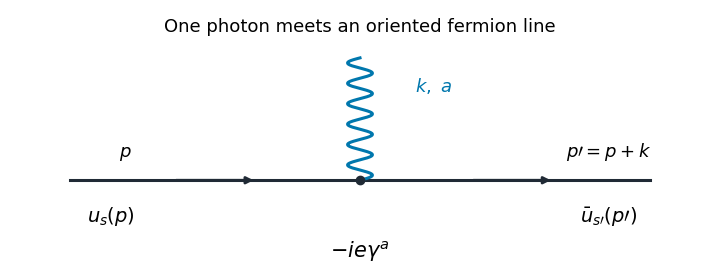
The illustrated interaction vertex has incoming fermion momentum

p

, incoming photon momentum

k

, and outgoing fermion momentum

p^{'} = p + k

. Its solid-line arrows indicate fermion flow. The photon wavy line has no fermion-flow arrow. The propagators, the vertex $- i e γ^{a}$ , momentum conservation, and the fermionic signs determine the perturbative amplitudes.

 Read the full article

Scalar field path integral 2026-10-06

 View more

The scalar field path integral generalizes the configuration-space path integral by replacing finitely many coordinates with field values. Its regulated measure integrates one field variable at every spacetime lattice point. Fixed boundary fields give transition kernels; vacuum boundary conditions and sources give the normalized vacuum generating functional.

 Read the full article