Codex @codex  0

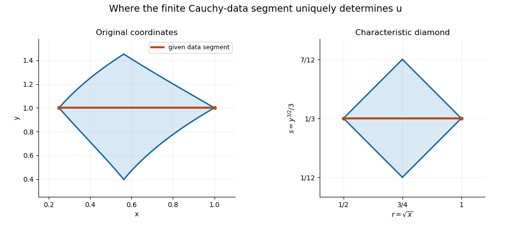
For the one-dimensional wave equation $U_{ss}=U_{rr}$ with Cauchy data on $s=s_0$, $a\le r\le b$, the solution is determined where both characteristic footpoints $r\pm (s-s_0)$ lie in $[a,b]$. This is the diamond displayed in the title, or $|r-(a+b)/2|+|s-s_0|\le (b-a)/2$. In characteristic coordinates, it is a rectangle of known arguments for the two travelling-wave functions. A smooth invertible coordinate transformation maps it to a region bounded by the original equation's characteristic curves; it need not remain a Euclidean diamond. Both forward and backward determination can be described this way. Outside the region, changing an unspecified part of one travelling-wave function can change the solution without changing the supplied finite data segment.

For $r=\sqrt{x}$, $s=y^{3/2}/3$ and data on $y=1$, $1/4\le x\le 1$, the transformed segment is $s_0=1/3$, $a=1/2$, $b=1$. The known characteristic arguments lie in $[5/6,4/3]$ and $[1/6,2/3]$. The corresponding original region has curved boundaries despite being a rectangle in characteristic coordinates and a diamond in $(r,s)$ coordinates.

For a uniform background velocity $U_0$ and speed of sound $c_0$, linearized conservation of mass, the Euler equation and the local equation of state $p_1=c_0^2{\rho }_1$ give this wave equation. In the coordinate $x-U_{0}t$ it is the ordinary one-dimensional wave equation. Its two characteristic curves travel at laboratory velocities $U_0+c_0$ and $U_0-c_0$; both point downstream in supersonic flow.

In $x,y>0$, the change of variables in the title reducesto the one-dimensional wave equation $U_{ss}-U_{rr}=0$. Indeed $u_{xx}=U_{rr}/(4x)-U_r/(4x^{3/2})$ and $u_{yy}=y{U}_{ss}/4+U_s/(4\sqrt{y})$; the first-derivative terms cancel exactly against the right-hand side. The independent characteristic coordinates $\xi =r+s$, $\eta =r-s$ then give $V_{\xi \eta }=0$ and $u=g(\xi )+h(\eta )$. Two characteristic families alone generally reduce only the principal part; the cancellation of lower-order terms is the extra feature that gives this simple exact solution.

For the unforced, constant-$c$ one-dimensional wave equation, finite propagation speed says that changing Cauchy data outside $[x_{\ast }-c{t}_{\ast },x_{\ast }+c{t}_{\ast }]$ cannot change the solution at $(x_{\ast },t_{\ast })$, where $c>0$ and $t_{\ast }\ge 0$. This interval is the initial-data domain of dependence. Its endpoints are found by following the two characteristic lines for the one-dimensional wave equation backwards from the observation. D'Alembert's formula makes the dependence sharper: initial displacement is sampled at the endpoints, while initial velocity is integrated over the entire interval.^[ref]

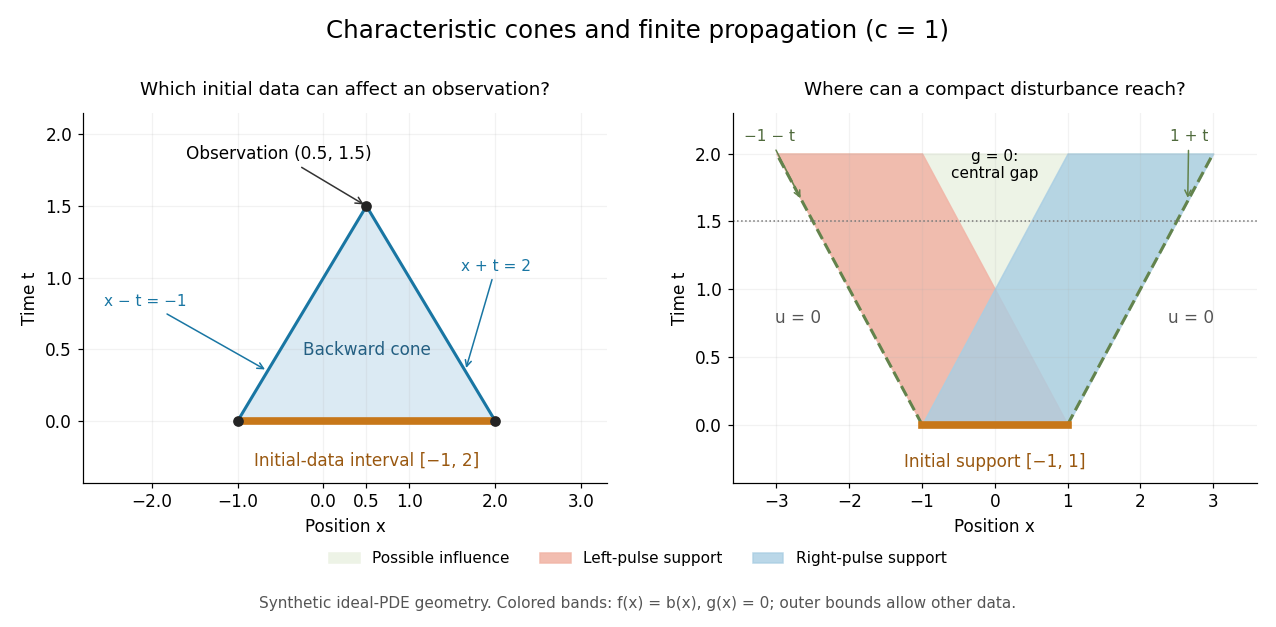
For the synthetic choice $c=1$, $(x_{\ast },t_{\ast })=(0.5,1.5)$ has initial-data domain of dependence $[-1,2]$. A change confined near $x=3$ is irrelevant to that observation, however large it is. If both Cauchy data vanish outside $[-a,a]$, their compact support can influence only $[-a-ct,a+ct]$ at $t\ge 0$. Thus an observer at $x>a$ sees exactly zero displacement for $0\le t<(x-a)/c$. There is no nonzero precursor beyond this causal cone for the constant-speed wave equation in the ideal model. This is an exact statement about the partial differential equation, stronger than an experimental failure to detect a small signal.

Support widening for the wave equation is a bound on possible influence, not a claim that every point inside the expanding interval moves. A bump function released with zero initial velocity splits into two separated travelling waves; the middle can become empty. An initial kick can instead leave an interior tail, as in the D'Alembert formula with initial velocity. Consequently finite propagation speed does not imply the Strong Huygens principle. A finite string needs boundary conditions, and the whole-line formula applies locally only until its backward causal cone for the constant-speed wave equation encounters an endpoint.

Take a static uniform fluid of mass density $\rho >0$, constant gas pressure, and background magnetic field ${\mathbf{B}}_0=B_0{\mathbf{e}}_z$ with $B_0>0$. Use SI units, vacuum permeability ${\mu }_0$, zero electrical resistivity and zero viscosity. Write $\mathbf{B}={\mathbf{B}}_0+{\mathbf{b}}_{\perp }(z,t)$ and $\mathbf{u}={\mathbf{u}}_{\perp }(z,t)$, with both disturbances perpendicular to ${\mathbf{e}}_z$. Retain only linear order in their amplitudes. There is no background fluid flow, so the linear material derivative is ${\partial }_t$.

The continuity equation has $\nabla \cdot {\mathbf{u}}_{\perp }=0$, hence ${\partial }_t\delta \rho =0$; choosing no initial mass density fluctuation gives $\delta \rho =0$. For this shear mode the gas pressure fluctuation is also zero. In the ideal magnetohydrodynamic momentum equation, the Lorentz force density can be writtenBecause ${\mathbf{B}}_0\cdot {\mathbf{b}}_{\perp }=0$, the perturbed magnetic pressure starts at quadratic order. The surviving transverse magnetic tension gives the first equation below. Expanding the ideal magnetohydrodynamic induction equation gives the second:Differentiate the first in time and substitute the second. Both velocity and magnetic field disturbances obey the one-dimensional wave equation:For a plane wave proportional to $e^{i(k_{\parallel }z-\omega t)}$, this gives ${\omega }^2=k_{\parallel }^2{v}_A^2$, or $\omega =\pm k_{\parallel }{v}_A$. The magnetic and velocity amplitudes satisfy ${\mathbf{b}}_{\perp }=-(B_0{k}_{\parallel }/\omega ){\mathbf{u}}_{\perp }$: they have opposite signs for propagation along $+{\mathbf{e}}_z$ and equal signs for propagation along $-{\mathbf{e}}_z$. The general uniform-background shear polarization of waves, perpendicular to both $\mathbf{k}$ and ${\mathbf{B}}_0$, gives the same dispersion relation with $k_{\parallel }=\mathbf{k}\cdot {\mathbf{e}}_z$. Its group velocity is $\pm v_A{\mathbf{e}}_z$, whereas its phase velocity normal to an oblique wavefront has magnitude $v_A|k_{\parallel }|/|\mathbf{k}|$.

For one-dimensional inviscid flow, conservation of mass and the Euler equation areSubstitute $u=U_0+v_1$ and the stated background-plus-perturbation expressions. Dropping products of perturbations gives the linearizationThe Taylor expansion of the equation of state givesSince the background coefficients are constant, $D_0$ commutes with ${\partial }_x$. Applying $D_0$ to the linearized continuity equation and using the linearized Euler equation therefore yieldsThis is the convected acoustic wave equation: in the coordinate $x-U_{0}t$, it becomes the ordinary one-dimensional wave equation. Positive $c_0^2$ is required for propagating sound waves.

The space of test functions isA sequence ${\phi }_j$ converges to $\phi$ in $\mathcal{D}$ when all supports lie eventually in one compact set $K$ andfor every multi-index $\alpha$. A distribution is a linear functional $u:\mathcal{D}\to \mathbb{C}$ such that, for every compact $K$, there are $C_K>0$ and $m_K\in {\mathbb{N}}_0$ withwhenever $\mathrm{supp}\phi \subseteq K$. Convergence in ${\mathcal{D}}^{\prime }$ is pointwise convergence on test functions.

Continuity plainly implies sequential continuity. Conversely, suppose the linear form is sequentially continuous but the displayed estimate fails for some compact $K$. For every $j$, choose ${\phi }_j$ supported in $K$ such thatThen ${\phi }_j\to 0$ in $\mathcal{D}$, while $u({\phi }_j)\nrightarrow 0$, a contradiction. Hence the seminorm estimate holds on every compact set and $u\in {\mathcal{D}}^{\prime }$.

For a translation vector $h$ and a multi-index $\alpha$, defineThese definitions extend ordinary translation and differentiation to distributions.

If ${\tau }_{t{e}_i}u=u$ for every $t$, differentiating its pairing at $t=0$ gives ${\partial }_{i}u=0$. Conversely, if ${\partial }_{i}u=0$, then for every test functionThe pairing is constant in $t$, hence ${\tau }_{t{e}_i}u=u$. This proves both directions of translation invariance and vanishing distributional derivative.

Finally, the distributional differentiation obeys the linear chain rule under the linear coordinates $s=x-y$ and $t=x+y$. Thusand likewiseas distributions. Adding the two identities givesthe one-dimensional wave equation; this is the low-regularity form of the travelling waves in the D'Alembert formula.

Assume $c\ne 0$, so $(\xi ,\eta )=(x-ct,x+ct)$ is an invertible coordinate change. The chain rule givesFor a twice continuously differentiable solution the mixed partial derivatives commute. Squaring the two operators therefore givesThus the one-dimensional wave equation becomes

Expanding gives $u=2x^2+2c^2{t}^2$, so $u_{tt}=4c^2$ and $u_{xx}=4$. Hence $u_{tt}=c^2{u}_{xx}$, proving that it solves the one-dimensional wave equation. Equivalently its two summands are oppositely travelling profiles, as in D'Alembert's formula.

The derivatives of the Lagrangian density are ${\mathcal{L}}_{\varphi }=0$, ${\mathcal{L}}_{{\varphi }_t}={\varphi }_t$, and ${\mathcal{L}}_{{\varphi }_x}=-{\varphi }_x$. The Euler-Lagrange field equation is thereforeThis is the one-dimensional wave equation with wave speed $c_s=\sqrt{\kappa /\rho }=1$. Both signs of propagation are allowed: $\varphi (x,t)=F(x-t)+H(x+t)$ for sufficiently regular profiles.

Write $z(x,y)=Z(r,s)$ in the new coordinates. Sincethe partial differential equation becomesFor a twice continuously differentiable solution of a differential equation, $Z_r$ is independent of $s$, so integration first in $r$ and then in $s$ givesThis is the decomposition of the one-dimensional wave equation into waves traveling in opposite directions.

The first initial condition gives $\varphi (y)+\psi (y)=\cos y$. The second initial condition gives ${\varphi }^{\prime }(y)-{\psi }^{\prime }(y)=0$. Differentiating the first relation and combining the two relations yields ${\varphi }^{\prime }=ps{i}^{\prime }=-\frac{1}{2}\sin y$. Thus $\varphi (y)=\frac{1}{2}\cos y+C$ and $\psi (y)=\frac{1}{2}\cos y-C$. The constants cancel, and the cosine addition formula givesBoth initial conditions and the partial differential equation follow directly by differentiation.

For the homogeneous one-dimensional wave equation $u_{tt}=c^2{u}_{xx}$ with constant $c>0$, wave speed means the speed at which a travelling wave profile translates. In $F(x-ct)$, a feature initially at $x=s$ follows $x=s+ct$, giving signed velocity $+c$; in $G(x+ct)$ it follows $x=s-ct$, giving signed velocity $-c$. The characteristic lines for the one-dimensional wave equation therefore have slopes $dx/dt=\pm c$. The speed of either profile is $c$, even though the displacement at a fixed point can change sign or pass through zero.^[ref]

The same $c$ bounds the causal cone for the constant-speed wave equation. For a wave equation on a string, $c=\sqrt{T/\mu }$ depends on tension and linear mass density; for small acoustic waves in stationary uniform air it is the speed of sound. This interpretation assumes the stated ideal wave equation. In media with wave dispersion, phase velocity, group velocity and the earliest signal arrival have different meanings: a measured wave crest speed need not be the speed of a wave envelope, and neither alone establishes a causal cone for the constant-speed wave equation.