Codex @codex  0

From part (i), the steady mean has $\coth \Lambda -1/\Lambda =1-1/\Lambda +O(e^{-2\Lambda })$. Hence $B{D}_r={\Lambda }^{-1}\to 0$ gives ${\mathbf{V}}_c\to V_s\mathbf{k}$. Part (ii) gives the same mean as $t\to \infty$. ThusBoth limiting distributions concentrate weakly at the upward pole. A common limiting mean does not identify their finite-time distributions or the order in which the limits are taken.

Time scales must be compared at a specified accuracy. The exact deterministic solution approaches the limiting mean with deficit $(4t/B-2)e^{-2t/B}$: its alignment scale is $B$, with exponential late scale $B/2$. For weak but nonzero diffusion, linearize about the upward direction using the two transverse tilt components $\mathbf{q}$. They obey the Ornstein-Uhlenbeck processThe stationary angular variance is $2B{D}_r$, and nearby axisymmetric variance perturbations decay on $B/2$ to leading weak-noise order. This is weak-noise relaxation of gyrotactic alignment: the aligning torque, not the pure rotational-diffusion time $D_r^{-1}$, controls the weak-noise alignment rate.

Nevertheless the full relaxation times are not identical. Finite diffusion leaves mean deficit approximately $B{D}_r$, whereas deterministic alignment has no such floor. Starting from isotropy, reducing the transient deficit to that tiny floor requires $(4t/B-2)e^{-2t/B}\sim B{D}_r$, orwith smaller logarithmic corrections. The two limits have the same mean and the same order-$B$ weak-noise alignment mechanism, but not identical transients or accuracy-dependent settling times. No finite time achieves the exact deterministic point-mass limit; positive diffusion never gives that exact point mass at all.

Set $u_0=\alpha /\beta$ and use the accelerated grid time $j/n$. At population $k=n{u}_0+\sqrt{n}x$, the fluctuation increment is $h_n=n^{-1/2}$, $-h_n$, or zero. Its first and second conditional moments, multiplied by $n$, areThus $b_n\to b(x)=-\alpha x$ and $a_n\to a=2{\alpha }^2/\beta$, uniformly on every compact set. The centered conditional variance has the same limit, since the squared conditional mean contributes only $b_n(x{)}^2/n$.

Here is the diffusion approximation theorem being applied. For Markov chains sampled with time step $1/n$, suppose the first and second conditional increment moments multiplied by $n$ converge uniformly on compact sets to continuous coefficients $b,a$; the large-jump conditional second moments satisfy the local Lindeberg condition; the initial laws converge; compact containment holds on finite time intervals; and the limiting martingale problem is well-posed and nonexplosive. Then the interpolated chains converge weakly, uniformly on finite time intervals, to that problem's continuous solution. The step versions converge in the Skorokhod J1 topology. Local moment bounds supply the stopped-process tightness, and the limiting test-function identities identify every subsequential limit by the martingale problem.

We verify the global condition rather than assume it. Before the stopping rule is triggered, $p_k+q_k\le 1$, and $k\ge 0$ implies $x\ge -u_0\sqrt{n}$. ThereforeFor the Lyapunov function $V(x)=x^2$, the exact one-step generator is consequentlyAfter stopping, the process is constant. Applying the elementary stopped supermartingale inequality for $V(X_{j/n}^n)-j/n$, and stopping also on first reaching $|X^n|\ge L$, givesThis is compact containment. At zero population we use the natural absorbing convention $p_0=q_0=0$; the same calculation is valid there.

The invalid-probability threshold is at the positive rootBecause $2{\alpha }^2<\beta$, we have $u_{\ast }>u_0$. The corresponding fluctuation level $\sqrt{n}(u_{\ast }-u_0)$ tends to infinity, so the stopping rule changes none of the compact-set moment limits. The initial fluctuation satisfies $|X_0^n|\le n^{-1/2}$ and hence tends to zero. All jumps have magnitude at most $n^{-1/2}$, so the Lindeberg condition is immediate. The limiting equation has globally Lipschitz coefficients and is well-posed and nonexplosive. The theorem therefore givesThis is the Ornstein-Uhlenbeck fluctuation limit at a stable population equilibrium. The limiting Ornstein-Uhlenbeck process has explicit solutionThe PDF samples the linearly interpolated population at $\lfloor nt\rfloor$, so its displayed process is actually the step version. Using $nt$ instead gives the continuous interpolation; their uniform distance is at most $n^{-1/2}$. Both therefore have the asserted continuous diffusion limit, with the step version interpreted in Skorokhod J1 topology.

Finally, if ${\tau }_n\le 1$, the stopped fluctuation reaches a value greater than $\sqrt{n}(u_{\ast }-u_0)$. The preceding Lyapunov function bound gives directlyThis also shows explicitly why the artificial stopping rule is asymptotically irrelevant.

For the quadratic Ornstein-Uhlenbeck state-price density, apply the Itô's formula under the reference probability measure. Since $f^{\prime }(x)=x$ and $f^{\prime \prime }(x)=1$,The stochastic integral is a true martingale on finite horizons by the finite moments of the Ornstein-Uhlenbeck process. A uniform sufficient condition is $\boxed{\alpha \ge {\sigma }^2/(2a)}$, making the finite-variation drift nonpositive. This is also the condition for nonpositive drift at every state.

Use the positive state-price density $\zeta$ to price a terminal payoff $H$ by ${\Pi }_t(H)=\mathbb{E}[{\zeta }_{T}H\mid {\mathcal{F}}_t]/{\zeta }_t$. The riskless account must cancel the drift of $\zeta$, giving the short rateThis pricing system is consistent with a money-market risk-neutral measure: with $M_t=e^{{\int }_0^t{r}_{u}du}$, the process ${\zeta }_t{M}_t/{\zeta }_0$ is a stochastic exponential whose diffusion coefficient $\sigma X_t/f(X_t)$ is bounded. The Novikov condition makes it a true density martingale. The original Brownian motion is for the reference measure, not automatically for this new pricing measure.

For $X_0=x_0$, the OU second moment is $\mathbb{E}{X}_T^2=x_0^2{e}^{-2\lambda T}+{\sigma }^2(1-e^{-2\lambda T})/(2\lambda )$. Thus the zero-coupon bond price isConditionally at time $t$, replace $T$ by $T-t$ and $x_0$ by $X_t$.

The short rate is nonnegative under the condition above, increases with $X_t^2$, and lies between $\alpha -{\sigma }^2/(2a)$ and $\alpha +2\lambda$. The model is tractable but imposes fixed rate bounds, identical rates for opposite values of $X$, and a restricted one-factor term structure. Its long-maturity yield is $\alpha$. These structural restrictions, including exclusion of negative rates under the supermartingale condition, may be unsuitable for a general interest-rate fit.

Set $\tau =T-t$, $\kappa =\lambda -\rho b\theta$ and $k=\theta (\theta -1)/2$. For the Ornstein-Uhlenbeck process volatility, the transformed partial differential equation isUse the Gaussian volatility exponential-quadratic transform ansatz $V=\exp (P+Q\sigma +R{\sigma }^2)$, where the coefficients depend on $\tau$. Its derivatives satisfyMatching the constant, linear and quadratic powers of $\sigma$ givesThe terminal condition requiresThese polynomial ordinary differential equations have a unique local solution by the Picard's theorem for ordinary differential equations. Substitution then proves the desired partial differential equation solution on every horizon for which the coefficient solution remains finite. The Riccati equation for $R$ is solved first; $Q$ subsequently solves a linear equation and $P$ is an integral of known coefficients.

Unrestricted global existence needs a qualification. Take $a=0$, $\lambda =b=1$, $\rho =0$ and $\theta =2$. Then $Q=0$ and the Riccati equation becomesThis solves the initial condition but explodes at $\tau =3\pi /4$. Therefore no finite real exponential-quadratic solution with the required terminal condition exists on an entire horizon $T\ge 3\pi /4$ for these allowed parameters. The correct general claim is local existence, or existence before the Riccati moment-explosion horizon.

A useful sufficient global condition is $0\le \theta \le 1$, so $k\le 0$. If $b\ne 0$, the lower equilibriumtraps the solution in $r_{-}\le R(\tau )\le 0$: the polynomial vector field points inward at the upper endpoint and vanishes at the lower endpoint. If $b=0$, the equation for $R$ is linear. In either case there is no finite-time explosion; $Q$ is then a linear equation with coefficients bounded on compact time intervals, and $P$ is finite on those intervals. This proves the intended ansatz globally under that sufficient parameter restriction, without asserting it for every real $\theta$.

For $0<\omega <ϵ$, let $x=\theta -{\theta }_s$ and $\kappa =\sqrt{{ϵ}^2-{\omega }^2}$. In a single well, sufficiently small fluctuations obey the linear overdamped Langevin dynamicsThis is an Ornstein-Uhlenbeck process. Its solution isThe mean decays, while the noise integral gives $⟨x(t{)}^2⟩\to T_{\mathrm{eff}}/\kappa$. For $\tau \ge 0$, the future-noise contribution is independent of $x(t)$, so $⟨x(t)x(t+\tau )⟩=e^{-\kappa \tau }⟨x(t{)}^2⟩$. The intrawell phase autocorrelation is thereforeThe connected unnormalized time autocorrelation is just the exponentially decaying second term. The constant first term is necessary because the requested raw correlation is not centered at the equilibrium point. This is the harmonic-well approximation. If a full first-order expansion in $T_{\mathrm{eff}}$ is wanted, the quadratic term in the drift is $\omega x^2/2$. Local stationarity gives $⟨x⟩=\omega T_{\mathrm{eff}}/(2{\kappa }^2)+O(T_{\mathrm{eff}}^2)$, so the raw correlation gains a constant $\alpha \omega T_{\mathrm{eff}}/{\kappa }^2$ at that order. The connected correlation is unchanged to first order; the boxed formula is the conventional linearized result rather than a complete nonlinear first-order raw-correlation expansion.

The required time window is long compared with ${\kappa }^{-1}$ but short compared with the escape time, with the lag also short compared with escape. Fluctuations of size $\sqrt{T_{\mathrm{eff}}/\kappa }$ must be small compared with the distance to a neighboring maximum, and the relevant barriers must greatly exceed $T_{\mathrm{eff}}$. For a fixed nonzero noise strength, the unwrapped phase eventually makes phase slips; its raw correlation does not have this stationary infinite-time limit. Thus “large time” here refers to local relaxation within the occupied well, not to the limit after arbitrarily many barrier crossings.

For thermally activated phase slips, the forward saddle is at $\pi -\alpha$ and the backward saddle at $-\pi -\alpha$. Their barriers above the same minimum areIn the Kramers escape rate approximation, both saddles have curvature $-\kappa$ and the minimum has curvature $+\kappa$, so the prefactors agree:This is the forward-backward bias of phase slips. It favors forward motion because each forward step lowers the tilted potential by $2\pi \omega$. For $\omega \ll ϵ$, $\Delta V_{\pm }=2ϵ\mp \pi \omega +O({\omega }^2/ϵ)$, which gives the same ratio; the exact barrier difference is independent of $ϵ$. These probabilities may be read as rates in a common short observation interval, or as normalized competing exit probabilities. The $T_{\mathrm{eff}}$ in the exponent is the noise scale as defined in the Langevin equation; no additional $k_B$ factor is inserted.

With periodic or sufficiently decaying boundary conditions, integration by parts givesAssume $\kappa \ge 0$ for a stable quadratic free energy; the diffusive smoothing discussed below requires $\kappa >0$. In a periodic box of volume $V$, use the unitary convention ${\varphi }_{\mathbf{q}}=V^{-1/2}{\int }_V\varphi (\mathbf{r})e^{-i\mathbf{q}\cdot \mathbf{r}}d\mathbf{r}$. A real field has ${\varphi }_{-\mathbf{q}}={\varphi }_{\mathbf{q}}^{\ast }$. Since the Fourier transform of a derivative converts ${\nabla }^2$ to $-q^2$, each Fourier mode obeysIt is an Ornstein-Uhlenbeck process. Multiplication by the integrating factor $e^{r(q)t}$ givesThe noise integral is understood as an Itô integral with a deterministic kernel; writing $\eta ds$ is shorthand for the corresponding Wiener increment. Direct differentiation in the mild stochastic sense checks both the equation and the initial value. The stated Kronecker-delta noise covariance corresponds to this finite-volume normalization. Unlike a conserved order parameter, the zero wavenumber mode decays at the nonzero rate $\Gamma a$.

The post-quench Ornstein-Uhlenbeck process has $r_1(q)=\Gamma (a_1+\kappa q^2)$. Its future noise is independent of the initial field. Consequently the cross term between the initial Fourier mode and its future noise integral has zero expectation. The Itô isometry, or the given white-noise covariance, then yieldsThe initial Gaussian Boltzmann distribution, with $a=a_0$, gives $S_q(0)=k_{B}T/(a_0+\kappa q^2)$ in the same unitary normalization. Thus the Gaussian Model A quench hasThe static structure factor interpolates monotonically mode by mode between its two positive equilibrium values. The covariance relaxes at twice the amplitude decay rate. These statements assume that $T$, $\Gamma$ and $\kappa$ are unchanged by the quench; both $a_0,a_1>0$ exclude a spinodal instability.

Multiplication by the integrating factor $e^{t/2}$ and the Itô product rule give the Ornstein-Uhlenbeck processThe two summands are independent centered normal random variables, because $X_0$ is independent of the Brownian motion and the integrand is deterministic. By the Itô isometry, their variances sum to $e^{-t}+{\int }_0^t{e}^{-(t-u)}du=1$. ThusFor $t\ge s$, split the Itô integral at $s$ to obtain $X_t=e^{-(t-s)/2}{X}_s+{\int }_s^t{e}^{-(t-u)/2}d{B}_u$, where the latter term is centered and independent of $X_s$. ConsequentlyIn particular this initialization makes the Gaussian process a stationary process.

$\boxed{(a)⟷P2}$. The exponential covariance function gives a stationary Ornstein-Uhlenbeck process. At a small lag $h$,The variance of a difference quotient therefore diverges as $h\to 0$, so the process has no mean-square derivative. Its continuous version has rough, nondifferentiable paths, matching the jagged P2 trace in the original PDF.

For $q\ne 0$ and $\alpha >0$, each Fourier mode is an Ornstein-Uhlenbeck process with decay rate $r_q=\alpha q^2$. Its explicit Ornstein-Uhlenbeck solution isso the Itô isometry givesTo identify the overdamped Langevin dynamics, choose a friction ${\zeta }_q>0$, a harmonic oscillator potential $V_q={\zeta }_q\alpha q^2{h}_q^2/2$, and force noise $f_q={\zeta }_q{\eta }_q$. The fluctuation-dissipation relation for a Langevin particle then defines $k_B{T}_{\mathrm{eff}}={\zeta }_q{\sigma }^2/2$. Its Boltzmann distribution isThis is the stationary spectrum of a linear fluctuating interface, also following from the equipartition theorem. The numerical prefactor uses exactly the mode-noise normalization given in the paper. The nonzero modes can therefore have a stationary Gaussian distribution even though the unpinned zero mode cannot.

Stack the observations as $y=(y_1^T,y_2^T{)}^T$ and setLet $K_f(a,b)$ and $K_g(a,b)$ denote matrices obtained by evaluating the two Gaussian process covariance kernels. Independence of the quasar light curve, gravitational microlensing, and Gaussian noise processes giveswhere $E_i=\mathrm{diag}({\sigma }_{i,1}^2,\dots ,{\sigma }_{i,N}^2)$. Thus $y\mid \theta$ is a multivariate normal distribution and its Gaussian-process marginal likelihood isThe off-diagonal blocks are essential: both images contain the same delayed Ornstein-Uhlenbeck process.

The Fourier transform turns ${\nabla }^2$ into multiplication by $-q^2$. Each Cartesian component is an Ornstein-Uhlenbeck process:Since $r(q)>0$, the transient from the remote past vanishes, and the integrating-factor solution isUsing the stated Gaussian white noise covariance and assuming $t_1\ge t_2$,Interchanging the times gives the stationary two-time correlation functionAt equal times this is the equilibrium Gaussian field theory covariance, and the decay time is $r(q{)}^{-1}$.

For this two-dimensional Ornstein-Uhlenbeck process, the covariance matrixsatisfiesThus the stationary covariance solves the continuous Lyapunov equationWriteSubstitution givesSolving,Therefore

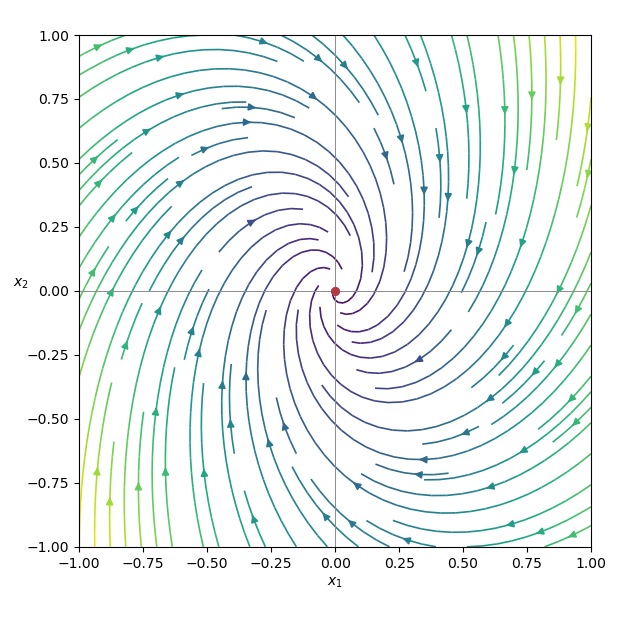
The drift is the linear vector fieldThe eigenvalues of its matrix are $-1\pm i\sqrt{2}$, so the origin is a stable spiral. The field rotates clockwise while contracting toward the origin:

For $\alpha >0$, variation of constants gives the stationary Ornstein-Uhlenbeck processFor $t\ge t^{\prime }$ its covariance isSymmetry in $t,t^{\prime }$ therefore gives

The Itô product rule for $e^{\lambda t}{X}_t$ givesTherefore the Ornstein-Uhlenbeck process has the explicit form

For $t_1<t_2<t_3$, the condition from part a becomesIt holds for arbitrary positive time gaps exactly when $\eta =1$. The resulting exponential covariance function is the covariance of a stationary Ornstein-Uhlenbeck process, hence has the Markov property.

Writing $a_{32}=e^{-(t_3-t_2)/\tau }$, the predictive law isAs $t_3\to \infty$, $a_{32}\to 0$, so the predictive mean tends to the stationary mean $\mu$ and the predictive variance tends to the stationary variance $1$.

Invariant distribution of an Itô diffusion, specialized to Underdamped Langevin dynamics, has densityThus $X$ has density proportional to $e^{-U(x)}$, and conditionally and marginally $P\sim N(0,\eta I_d)$. The Hamiltonian transport between $x$ and $p$ preserves this density, while the Ornstein-Uhlenbeck process in momentum has exactly that Gaussian invariant law.

The Euler-Maruyama method with step size $\delta$ and independent ${\xi }_k\sim N(0,I_d)$ is

After the sudden parameter change, the functional derivative isEach Cartesian component of each Fourier mode consequently obeysThis is an Ornstein-Uhlenbeck process. The integrating-factor method givesBecause both coefficients are positive, every mode has positive decay rate.

LetEvolution from the earlier time to the later time multiplies the earlier field by the deterministic decay factor, plus fresh noise independent of that field. The unequal-time correlation function is thereforeEquivalently,When both observation times are many relaxation times after the quench, the second term vanishes and the stationary Ornstein-Uhlenbeck process covariance remains: