Past exam of the chemistry course of the year 4 of the natural sciences course of the University of Cambridge / 2022 / Paper 3 / Section F

Take incidence from the left and set the reactant and product potentials to zero. The asymptotic scattering boundary conditions are $\psi =A{e}^{ikx}+B{e}^{-ikx}$ for $x<0$ and $\psi =F{e}^{ikx}$ for $x>a$, with $k=\sqrt{2mE}/\hslash$. There is no incoming wave from the product side. At each finite potential step, $\psi$ and $d\psi /dx$ are continuous for the same mass on both sides.

The probability current isFor the incident and transmitted travelling waves, $j_{\mathrm{in}}=\hslash k|A{|}^2/m$ and $j_{\mathrm{tr}}=\hslash k|F{|}^2/m$. Thus $P(E)=|F/A{|}^2$ here. If the asymptotic wave numbers differed, the ratio of outgoing to incoming velocities would also be required. Current conservation gives $P+|B/A{|}^2=1$ for a real nonabsorbing barrier.

Write $\psi =C{e}^{i\alpha x}+D{e}^{-i\alpha x}$ inside the barrier. Matching the wavefunction and derivative gives the four equationsFor sub-barrier energy the same equations hold by analytic continuation to imaginary $\alpha$. No coefficient solution is needed for these matching conditions.

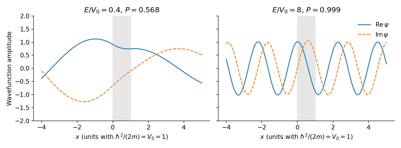
For $0<E<V_0$, put $\alpha =i\kappa$ with $\kappa =\sqrt{2m(V_0-E)}/\hslash$. Since $\sin (i\kappa a)=i\sinh (\kappa a)$, both signs in the quotient change andIt is finite and positive for nonzero incident energy and finite width: this is quantum tunnelling. In a thick barrier $P\simeq [16E(V_0-E)/V_0^2]e^{-2\kappa a}$. Inside, the scattering wave is a combination $C{e}^{-\kappa x}+D{e}^{\kappa x}$, not an isolated real decaying exponential; their complex coefficients allow a nonzero conserved current.

Let ${\kappa }_0=\sqrt{2m{V}_0}/\hslash$. As $E\to 0^{+}$, $\kappa \to {\kappa }_0$ while the large denominator term scales as $1/E$. HenceThe limit is linear in incident energy for fixed positive height and nonzero width. A below-barrier wave has nonzero penetration at finite energy, but that does not imply a finite zero-energy transmitted flux.

For $E\gg V_0$, expand the reciprocal to obtainRetain the exact $\alpha$ in the bounded oscillatory factor unless a further phase expansion is controlled. Reflection is small, with an oscillatory interference correction of order $(V_0/E{)}^2$. The wavefunction is nearly a travelling wave throughout; its wave number inside is slightly smaller than outside, so its wavelength is slightly larger there. The reflected wave adds weak standing-wave modulation on the incident side.

For fixed $V_0$ and $a$, $0\le {\sin }^2(\alpha a)\le 1$ while the multiplier of this bounded factor tends to zero as $E^{-2}$. Consequently $\boxed{\underset{E\to \infty }{\lim }P(E)=1}$, even though the sine factor itself does not have a limit. This is the high-energy classical transmission limit.

The classical transmission probability is $P_{\mathrm{cl}}(E)=\Theta (E-V_0)$; the convention exactly at the threshold does not affect a thermal integral. Below the barrier it is zero, whereas the quantum result permits tunnelling. Above the barrier it is one, whereas quantum reflection is generally nonzero except at transmission resonances. Both descriptions tend to unit transmission at arbitrarily high energy, and both have zero transmitted probability in the zero-energy limit for this positive barrier.

With $\beta =1/(k_{B}T)$ and a consistently normalized reactant partition function $Q_r$, the one-dimensional channel formula isClassically the integral starts at $V_0$, givingAn infinite free reactant half-line has no finite canonical population, so define a reactant normalization length $L$, for which $Q_r=L\sqrt{m/(2\pi \beta {\hslash }^2)}$. Then $k_{\mathrm{cl}}=L^{-1}\sqrt{k_{B}T/(2\pi m)}{e}^{-V_0/(k_{B}T)}$. Equivalently $kL$ is a one-dimensional thermal flux per unit reactant density, with dimensions of velocity. A rate constant without either this normalization or a specified reactant well is not dimensionally complete.

Choose a reaction coordinate $s(q)$ that is negative in the reactant region and positive in the product region; $s=0$ defines a dividing surface. With unnormalized canonical phase-space averaging, defineThe signed initial flux $\delta (s)\dot{s}$ counts both directions, while the later side function tests product commitment. The rate is $k=C_{fs}(t_{\mathrm{pl}})/Q_r$ on a plateau after microscopic recrossings have died away but before reactant depletion and global equilibration become important. The $t\to 0^{+}$ limit instead gives the transition-state-theory positive flux and can overcount trajectories that later return. A suitable dividing surface changes that early flux but not a correctly evaluated committed plateau rate. This correlation formulation provides the dynamical correction to a transition-state estimate.^[ref]

Take $s=x-x^{‡}$ with $0<x^{‡}<a$. A trajectory crossing to the right at the barrier top goes downhill on exit and cannot return in this model. Its initial Boltzmann weight contains $e^{-\beta V_0}$; negative-velocity trajectories are on the reactant side at the commitment time. ThereforeDividing by the same $Q_r$ gives the result in the energy-integral calculation. No width appears in the classical rate because every classically allowed trajectory passes through the flat barrier.

Put the dividing surface at $x^{‡}<0$. The immediate positive flux includes all positive momenta and gives $C_{fs}(0^{+})=1/(2\pi \hslash \beta )$, an overestimate. Trajectories with $p^2/(2m)<V_0$ hit the barrier, return across this surface, and cease contributing to the later product-side indicator. After their recrossing transient, only $p>\sqrt{2m{V}_0}$ survives:The exact rate is again unchanged; the transmission correction to the reactant-side transition-state estimate is $e^{-\beta V_0}$. The return time depends on surface placement and velocity, so the plateau means a timescale-separated limiting flux, not the claim that every trajectory has one identical finite recrossing time.

Let $z_{ij}$ be the input to output weight $w_j$ for datum $i$, including $z_{i0}=1$ for the bias. With identity output activation, $h_i=a_i={\sum }_j{w}_j{z}_{ij}$. The chain rule givesThe $z_{ij}$ are held fixed when differentiating an output-layer weight; they may be hidden-layer activations rather than raw descriptors. Hidden-weight derivatives require backpropagation through the preceding layers.

The printed PDF has a plus sign before the second logarithm. Differentiating that expression literally, with $h_i=\sigma (a_i)$ and $\partial h_i/\partial w_j=h_i(1-h_i)z_{ij}$, givesFor example, at $y_i=0$ it is $-h_i{z}_{ij}$, so minimizing this printed objective pushes the predicted probability of class one upwards rather than downwards; the objective is unbounded below as $h_i\to 1$. It is therefore not the usual binary cross-entropy.

If the second sign was intended to be negative, the standard negative log-likelihood is $-y_i\log h_i-(1-y_i)\log (1-h_i)$ and the derivative simplifies instead to $(h_i-y_i)z_{ij}$. Stating both cases preserves the actual question's algebra while identifying the apparent sign error. The logarithms here are natural; another base multiplies the gradients by its constant conversion factor.

For $K$ mutually exclusive classes, the output layer should provide $K$ nonnegative probabilities summing to one, with labels aligned consistently to output coordinates. A softmax activation on logits $a_k$ providesSubtracting ${\max }_{\ell }{a}_{\ell }$ from all logits before exponentiation preserves these probabilities and prevents numerical overflow. Categorical cross-entropy $-{\sum }_k{y}_k\log p_k$ is appropriate for one-hot or probabilistic class targets. Independent sigmoid outputs fit a different setting in which multiple labels can be present simultaneously and their probabilities need not sum to one.

Compose affine maps with nonlinear hidden activation functions, for example $h(x)=W_2\mathrm{ReLU}(W_{1}x+b_1)+b_2$. Several hidden units can respond to different linear combinations of input features; later units combine their responses to represent curved or piecewise-linear decision boundaries and interactions. A product interaction can be understood from $xy=[(x+y{)}^2-(x-y{)}^2]/4$: units approximating nonlinear functions of $x+y$ and $x-y$ can represent effects that no single additive linear fit captures.

Nonlinearity in hidden layers is essential: with only identity activations, repeated affine maps collapse to one affine map regardless of depth. Width and depth determine available representations; regularization, validation and suitable optimization are needed to learn useful rather than overfitted interactions. A nonlinear output activation alone applied to one linear score does not give an unrestricted model of feature interactions.

A multilayer perceptron usually connects every input unit of a layer to every output unit. For $n$ inputs and $m$ outputs its dense affine layer has $nm+m$ parameters, including biases. A convolutional layer instead applies small local filters with weight sharing across positions. A two-dimensional filter of size $k_h\times k_w$, with $C_{\mathrm{in}}$ input channels and $C_{\mathrm{out}}$ output channels, has $k_h{k}_w{C}_{\mathrm{in}}{C}_{\mathrm{out}}+C_{\mathrm{out}}$ parameters. The count does not increase with spatial height and width, although the activation storage and arithmetic do.

Local receptive fields and repeated layers capture increasingly extended patterns. translation equivariance follows from shared filters under compatible boundary conventions; pooling or global aggregation can help build invariance but a convolution alone is not generally translation-invariant. Flattening a large convolutional output into a dense head can reintroduce many parameters. For an unordered descriptor vector, a convolutional locality assumption must be justified rather than imposed merely because convolutional layers have fewer weights.