Solutions to the paper dated 5 June 2015.[ref]
Advanced Data Structures and Algorithms examination paper by the University of Oxford (2015). Cover, formal code A10399W1; question pages 2–3
All thirteen numbered subparts are treated. The original cover and both question pages have been checked, including the directions and labels of the flow network diagram. The binary counter and decimal counter analyses use the conventional all-zero initial state; the effect of allowing a different initial state is stated explicitly.The accounting method assigns each operation a charge, its amortized cost, that can differ from its actual cost. Cheap operations save the excess charge as credits associated with the data structure or its entries. An expensive operation spends these previously saved credits. The essential invariant is that the credit balance never becomes negative.
If the initial balance is zero, operation has actual cost , charge , and leaves balance , thenThus a nonnegative credit balance makes the total charge an upper bound on the total actual cost for every operation sequence. In particular, a constant time charge proves a linear time total. The argument is a deterministic amortized analysis; it requires no probability distribution on the operations. A nonzero initial balance must be included as an additive term in the bound.
Yes: starting from zero, increments of the decimal counter cost digit changes, uniformly in the number of digits. An increment changes the trailing digits equal to into and increases the next digit. Number digits from at the least significant end. Digit changes once every increments, so the exact number of changes isHere the floor function counts carries reaching each position, and the last equality sums a geometric series. Since digit changes on every increment, for . The loop tests and carry handling add only a constant amount per changed digit and per operation, giving the same time complexity.
An accounting method explanation is also possible. Charge two credits for each change of digit : one pays for that change and one joins a common bank. For increments the higher digits change at most times, so their costs can be covered from that bank; the displayed prefix bound ensures that it never goes negative.
The formula allows wraparound modulo ; alternatively, restrict to increments before overflow. Initializing the array itself costs if that is counted separately. If the initial digits are arbitrary, the number of changes at position is at most , giving in Big O notation. Starting with all digits equal to makes the first increment cost , so the initial-state convention matters.
For an initially zero binary counter, bit changes precisely on increments whose indices are divisible by . Weighting each such change by gives the exact totalFor and , put . All summands with vanish; each of the other summands is at most . ThereforeThis is sharper than simply charging for each of all positions when is small. To show that the order is best possible, use for . For every ,Thus the asymptotic analysis gives a tight bound. If wraparound is excluded, , and this becomes , often written for . If wraparound is allowed and , it becomes . For , the cost is zero.
For completeness, the same conclusion cannot be asserted uniformly over arbitrary initial binary counter states. An initial value makes the first increment change every bit, costing . A general upper bound follows by replacing each floor function in the count by a ceiling function:To see the second inequality, split at : for , use , and for , use . For the worst initial-state cost is consequently . This qualification separates initialization from the usual amortized analysis starting at zero.
Use two permanent stacks, and , and one temporary stack, . At operation boundaries is empty. Maintain the representation invariant that the deque, read from front to back, is the top-to-bottom contents of followed by the bottom-to-top contents of . Thus the tops of and are the two accessible ends. Maintain their sizes using two counters, requiring only additional storage in Big O notation.
Adding at the front pushes onto ; adding at the back pushes onto . Removing at an end whose permanent stack is nonempty simply pops that stack. If both permanent stacks are empty, report an empty deque.
- Move the top elements of onto .
- Move all remaining elements of onto .
- Move all elements of back onto .
- Pop and return the top of .
The parked elements are the back half of the deque; the unparked elements are the front half. Moving the front half onto reverses their stack order and exposes the correct front element. Parking and restoring the back half reverses it twice, preserving its original order in . The temporary stack is empty again. For a back removal with empty, exchange the roles of and throughout. Rebalance approximately half the elements, so both ends retain accessible elements after a large transfer.
For the amortized analysis, count each push or pop as one unit and use the potential method withInitially the deque is empty, so , and is always nonnegative. An ordinary insertion or removal costs one unit and changes the size difference by at most one, giving amortized cost at most .
For a rebalancing removal, let . The parked half makes two transfers per element and the other half makes one; each transfer is a pop and a push. Including the final removal, the actual cost isBefore rebalancing the absolute size difference is . Immediately after the split it is at most , and after the removal it is at most . HenceSize tests and counter updates change only these constants. Summing the amortized costs and using nonnegative final potential proves amortized running time for all four operations, with three stacks and additional storage. An individual rebalancing operation can still take linear time in the current size.
A flow network is a finite directed graph with nonnegative flow network edge capacities , together with distinct source and sink vertices . A feasible flow in the nonnegative directed-edge convention is a function satisfying the capacity constraints and flow conservation:Its flow value is the net outflow at the source,which equals the net inflow at the sink by flow conservation.
A cut of a flow network is a partition of a set with and . Its cut capacity counts only directed edges leaving :The net flow across the cut of a flow network subtracts flow on edges returning into , and equals .
For the following parts, a circulation with vertex demands has no exceptional source or sink in the original directed graph. Instead it satisfies net inflow minus net outflow equal to at every vertex. Thus positive demands consume flow, and negative demands supply flow.
Write flow balance using the positive-inflow conventionRemove the lower bounds on network flow by writing , where only is nonzero. Then , and its required flow balance isIn the order , the lower-bound contribution is , soThe resulting flow network edge capacities areAdd a new source with an edge of flow network edge capacity , and a new sink with edges and of flow network edge capacities and . A feasible flow saturating these new edges is equivalent to a solution for : ordinary flow conservation in the enlarged flow network produces exactly the residual supplies and demands above. All source and sink edges must be saturated, requiring flow value .
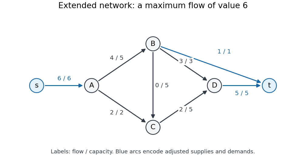
Extended flow network after removing the lower bound; labels show final flow divided by flow network edge capacity
. The auxiliary edges are blue. The displayed flow saturates the auxiliary source and sink edges, certifying that all adjusted demands are met. The original edge regains its four-unit lower bound only after this auxiliary problem is solved. Details.
Start the Edmonds–Karp algorithm at zero flow. Repeated breadth-first search in the residual network permits the following shortest augmenting paths; when paths tie, choose the one through first.
| Step | Augmenting path | Added flow | Total flow value |
|---|---|---|---|
The first augmenting path has three edges. Once is saturated, the next shortest possibilities have four edges, so steps and respect the breadth-first search rule. Each augmentation adds the usual backward edges to the residual network, though these particular augmentations need only forward edges. Now is saturated, so no further augmenting path exists. The cut of a flow network with source side has cut capacity , proving that the obtained flow is a maximum flow.
The original-edge values for are in the order . Restore the lower bound to obtainAll original capacity constraints hold, and meets its lower bound. The net inflows at are respectivelyThe original network therefore admits a feasible circulation with vertex demands.
For any feasible circulation with vertex demands, sum its defining flow balance over all vertices:Every directed edge contributes exactly once to the first sum, at its head , and exactly once to the second, at its tail . The two sums therefore contain exactly the same terms. They cancel, givingThis is global flow conservation: internal transport cannot create or destroy the total amount. Lower bounds on network flow and capacity constraints restrict which flows are feasible but do not affect the cancellation. The condition is necessary, not sufficient: insufficient flow network edge capacities can still prevent satisfying balanced demands.
For each user define its set of eligible ads byThis uses the intersection of demographic-group memberships: belonging to one advertised group suffices, because the eligibility condition is a set union. A user in several groups still receives at most one ad.
A direct algorithm is to process users independently. For user , scan ads until finding one for which some group belongs to both and . Assign that ad and stop processing this user. If no such ad exists, leave the user unassigned. There is no upper bound on the number of different users who can receive the same ad, so these decisions do not compete for an ad resource.
For correctness, every produced impression has a shared permitted group, and the stopping rule assigns at most one ad to each user. Conversely, a user with cannot receive an ad in any feasible solution. Since every other user can contribute at most one impression, every feasible solution has value at mostThe algorithm attains this bound, provingRepresent each membership set by a length- array of Boolean variables. Testing one user-ad pair costs , so all tests and input setup take time in Big O notation, which is polynomial time in all three parameters. For positive , this simplifies to .
A maximum flow formulation gives the same result if desired: add edges with flow network edge capacity , with flow network edge capacity exactly when , and with flow network edge capacity . By the integral max-flow theorem, an integral maximum flow selects valid impressions. Setting the last flow network edge capacity to would impose an extra restriction absent from this paper.
Using the standard maximum form of a linear program, writewhere , , , and . The inequalities are coordinatewise, and is the objective function. General linear programs can be put in this form: reverse the sign of a minimization objective function, reverse lower-bound linear inequalities, replace an equality by two opposite linear inequalities, and replace each unrestricted variable by the difference of two nonnegative variables. Some conventions instead call the equality-constraint version standard form; the convention here is the maximum-with-upper-bounds convention.
Introduce nonnegative slack variables . The equivalent slack form of a linear program isThe original variables are initially nonbasic and the slack variables basic. More generally, a slack form of a linear program specifies disjoint index sets and writesThus each basic variable and the objective function are expressed using only nonbasic variables. Setting all nonbasic variables to zero gives the associated basic solution, which is a feasible solution exactly when the resulting basic values are nonnegative. The slack form of a linear program does not itself require that initial basic solution to be feasible.
A vertex cover of an undirected graph is a subset containing at least one endpoint of every edge. The optimization version of the vertex cover problem minimizes ; the vertex cover decision problem asks whether a cover of size at most a given bound exists.
Let mean that vertex is selected. An integer program for minimum-size vertex cover isThe linear programming relaxation replaces by . The edge inequalities enforce coverage, and the objective function counts selected vertices in the integer program.
For a graph triangle with vertices , the three covering constraints areAdding them gives . Therefore the relaxed objective function is at least . The feasible solution attains that lower bound, soIn contrast, one vertex leaves the opposite edge uncovered and any two vertices cover all three edges, giving integer optimum . The example exhibits a genuinely non-integer optimal value, rather than merely a fractional feasible solution.
Assume job sizes and machine speeds , with at least one machine. Let be the amount of job assigned to machine , and let be the proposed makespan. Use the linear programThe first family of constraints assigns every job completely. The second bounds each machine's completion time by , since is equivalent to . It is a linear inequality because is an input constant. There is no integrality restriction: jobs are divisible as specified in this scheduling model.
To verify the formulation, any actual allocation defines the variables above, with equal to its largest completion time, and satisfies every constraint. Conversely, from a feasible solution, assign amount to machine and process its assigned pieces consecutively. Its total time is at most , so the linear program realizes the claimed makespan.
There is also a useful exact check. Put and . Summing machine constraints gives , so . Assigningmakes every machine's completion time , provingThis relies on the paper's divisible-work model, in which machine completion times depend only on total assigned size. If , the optimum is .
A feasible point is an extreme point solution of a linear program if it cannot be written as a nontrivial convex combination of two distinct feasible points. Explicitly, ifthen . Equivalently, lies in no open line segment joining two distinct feasible points. Being an extreme point concerns the feasible region; it does not by itself mean that optimizes the objective function.
Let be the given bipartite graph. A matching in a graph selects edges with no shared endpoint. For each edge , introduce an indicator for selection. The integer program for a maximum cardinality matching isIts linear programming relaxation iswith the same objective function. Explicit upper bounds may be included, but they already follow from a constraint at either endpoint.
We prove that every extreme point of is integral by showing that any feasible point with a fractional coordinate admits a two-sided perturbation. Given such an , form the fractional support graph with exactly those edges for which . This is a nonempty bipartite graph. A vertex incident to one of these edges cannot also meet an edge with value , because its incident sum would exceed .
First suppose contains a graph cycle. Choose a simple one, . Its length is even since is a bipartite graph. Define a nonzero vector by alternating along the graph cycle and putting on other edges. At each vertex on the graph cycle, the two changed coordinates have opposite signs, so its incident sum is unchanged. ChooseThen and are distinct feasible points: no coordinate leaves and all incident sums are unchanged. Since , it is not an extreme point.
Otherwise is a forest. Choose a connected component of a graph containing an edge, and a simple graph path in it between two tree leaves. Alternate along the graph path to define . Every internal vertex of the graph path still has unchanged incident sum, including any additional edges branching from it. At either endpoint, exactly one incident edge has fractional value; all other incident coordinates are , since a coordinate is impossible there. Thus each endpoint has strictly positive slack in its degree constraint. Choose smaller than these two slacks and smaller than every and along the graph path. Both and remain feasible: the endpoint sums can increase or decrease by , and the internal sums do not change. Again is the midpoint of distinct feasible points, contradicting extremality.
Both cases exclude fractional coordinates at an extreme point. ThereforeThe nonempty bounded linear polyhedron has an optimal extreme point for the stated linear function, so the relaxation yields a maximum cardinality matching. This is stronger than the existence of one integral optimum: it proves integrality of every extreme point. It does not claim that every optimal feasible point is integral; convex mixtures of distinct optimal matchings in a graph can be fractional.
Articles by others on the same topic
There are currently no matching articles.