Use Newtonian gauge with scalar metric perturbationsLet point from the observer toward the emitter, , and evaluate the unperturbed ray at . In the sudden-decoupling approximation the Sachs-Wolfe effect and its linear companions giveHere is the intrinsic photon monopole; is the emission gravitational redshift; the velocity term is the Doppler CMB anisotropy of the baryon-photon plasma; and the integral is the Integrated Sachs-Wolfe effect from evolving potentials during travel. The last two local terms are an observer monopole and dipole, removed when discussing the higher measured multipoles. Changing the direction convention reverses both velocity signs. A finite cosmological visibility function replaces the sharp emission surface by a weighted source integral.
For scale-invariant primordial potentials, is constant before transfer effects. In matter domination, the adiabatic superhorizon relation is , so the observable Sachs-Wolfe combination is . Its amplitude per logarithmic scale is therefore approximately independent of angle. In a flat geometry and , and projection gives the Sachs-Wolfe plateauBoth the intrinsic and gravitational emission terms have this leading large-angle scaling; they must be combined, not treated as unrelated random sources.
The Euler equation gives for the growing large-scale matter mode. Thus the Doppler amplitude grows roughly as relative to the large-scale potential amplitude, while its logarithmic power grows as , until acoustic dynamics and damping invalidate that simple estimate. On subhorizon pressureless scales the Poisson equation gives : the corresponding density amplitude has the often-used scaling. This is a matter-density estimate, not a universal small-angle photon-temperature law; the actual intrinsic photon source undergoes the oscillations in part(b). On superhorizon scales it instead has the constant-potential behavior just described.
The integrated source vanishes for constant linear potentials in pure matter domination. Potential decay during radiation domination or late accelerated expansion makes it nonzero. Its broad, slowly evolving sources favor large angular scales and give a potential-sized contribution there; crossings of many structures cancel progressively on small scales. Scale invariance alone fixes no universal power of angle for the integrated term: its time evolution and transfer functions are also required. Consequently the large-angle plateau, velocity-gradient enhancement and subhorizon density-gradient estimate describe distinct physical regimes, rather than one extrapolated power law across the whole spectrum.
For adiabatic initial conditions, the coupled photon-baryon fluid begins with a coherent displacement and approximately zero initial acoustic velocity. Neglecting slowly varying gravitational driving, its effective temperature satisfies an oscillator equation with phase , whereThus the Sachs-Wolfe combination has a dominant cosine phase, while the velocity has a sine phase. At last scattering, the first three temperature Cosmic microwave background acoustic peaks correspond approximately to : first compression, first rarefaction, and second compression of the initially displaced plasma in a potential well. Baryon inertia shifts the oscillator's equilibrium and enhances compressions relative to rarefactions, producing the familiar odd/even peak contrast. Potential decay and radiation driving alter the amplitudes, especially of the earliest peaks.
Adjacent displacement extrema differ by , soHere is the transverse comoving distance to last scattering; in a flat model it is . If is treated as constant, this reduces to . No numerical spacing is determined without a cosmological distance and sound horizon. Gravitational phase shifts, baryon loading and projection displace the exact peak locations from integer multiples of this spacing. These are primarily coherent density-plus-potential acoustic peaks; the label “Doppler peaks” does not mean the velocity term alone creates their sequence.
The first mechanism is Silk damping: finite photon mean free paths allow radiation to diffuse out of compressions, while velocity slip and radiation shear dissipate acoustic motion. A Fourier diffusion equation has , hence . For the polarization-inclusive tightly coupled plasma, a useful expression isThe positive scattering rate is , and is the baryon loading parameter. The two terms represent heat conduction from velocity slip and photon shear viscosity. The mode amplitude has an approximately Gaussian cutoff in ; power is suppressed by . The formula assumes tight coupling and slowly varying coefficients before decoupling.
The second mechanism is finite-width last-scattering damping. Photons emerge from a range of times and depths, so rapidly varying sources are averaged rather than observed at one sharply defined phase. Approximate the normalized cosmological visibility function by a Gaussian of width . For a radial plane-wave phase,The associated power factor is . An acoustic factor is likewise averaged, replacing by in the constant-sound-speed approximation. Thus fine radial structure and rapid acoustic time oscillations are suppressed once their phase changes substantially across the visibility width. This is an averaging effect after the perturbations exist; Silk damping physically erases them by diffusion. Angular projection and the evolving source determine the final isotropic damping envelope, so the radial dependence must not be silently discarded.
Thomson scattering generates linear Cosmic microwave background polarization when the incident radiation has a photon quadrupole. The cross-section prefers electric fields perpendicular to the scattering direction. Contributions from an isotropic field cancel, and a dipole alone does not supply the required spin-two angular pattern. Schematically the outgoing Stokes combination is proportional towhich selects the incident quadrupolar angular dependence. Tight coupling nearly isotropizes the radiation, making the quadrupole small; it develops when the photon mean free path becomes finite near decoupling. At leading tight-coupling order its size scales as .
The polarization is therefore weaker than the temperature anisotropy: a characteristic amplitude is of order a few percent to roughly ten percent of the temperature signal, or several microkelvin compared with temperature fluctuations of several tens of microkelvin on acoustic scales. This is an order-of-magnitude comparison, not a scale-independent ratio of every power-spectrum multipole.
The photon monopole follows the acoustic displacement, approximately ; the velocity sourcing the quadrupole follows . Hence polarization maxima occur near displacement zeros, between the main temperature peaks. In the leading coherent-oscillator approximation the shift is half the peak spacing, , although projection and gravitational driving modify exact locations. Scalar perturbations generate E-mode polarization at linear order, not B-mode polarization. Tensor perturbations and lensing can give B modes, and reionization generates an additional large-angle polarization feature.
Three distinct low-redshift nonlinear contributions are:
- The thermal Sunyaev-Zeldovich effect arises when hot cluster electrons inverse-Compton scatter the cosmic microwave background. Photons receive energy from the thermal electron distribution. With , the thermodynamic-temperature equivalent is , with Compton y parameter . This is a spectral distortion: a low-frequency decrement, a high-frequency increment, and a nonrelativistic null at , about217GHz for the present CMB temperature. Relativistic electron corrections shift the detailed spectrum and null.
- The kinetic Sunyaev-Zeldovich effect is the Doppler shift caused by scattering off the bulk motion of an electron cloud. At lowest order, . It can have either sign. Unlike the thermal effect, it has the spectrum of a small blackbody temperature shift: frequency independent in thermodynamic temperature units, or proportional to in intensity units.
- The Rees-Sciama effect arises from potentials changing during nonlinear collapse, accretion or motion of structures. Energy gained when a photon enters a well need not equal energy lost on departure. Its gravitational line-of-sight source is the nonlinear evolving-potential counterpart of the Integrated Sachs-Wolfe effect. It too is achromatic in thermodynamic temperature units, not a Compton spectral distortion. Linear potentials can be constant in a matter era while nonlinear potentials still evolve.
Gravitational lensing supplies another nonlinear modification by remapping pre-existing temperature and polarization patterns. It preserves the local blackbody spectrum; it does not generate temperature differences by lensing a perfectly isotropic background.
A low-frequency example is Galactic synchrotron emission: relativistic electrons spiral in the Galactic magnetic field and emit a broad nonthermal spectrum. In antenna-temperature units its approximate spectrum is with around3, varying with the electron population and sky direction. It is a major, often dominant contamination at frequencies below roughly20–40GHz; radio point sources and bremsstrahlung can contribute in the same low-frequency region.
A high-frequency example is Galactic thermal dust emission. Grains heated by starlight have approximate modified-blackbody spectrum , with grain temperatures of order tens of kelvin. Their emissivity-weighted emission rises rapidly through the microwave/submillimeter range and commonly dominates anisotropy contamination above roughly100–200GHz, especially at higher frequencies. Dusty extragalactic galaxies provide a related high-frequency foreground.
Synchrotron is the low-frequency contaminant and thermal dust the high-frequency contaminant. There is no universal crossover frequency at which either exceeds CMB anisotropy everywhere: sky masking, angular scale, polarization and source amplitude matter. Cleaner cosmological windows lie between these regimes, and multi-frequency observations distinguish the foreground spectra from a thermodynamic CMB temperature perturbation. The separation into low-frequency emission and high-frequency dust is also used in the Planck astrophysical-component products.
Use physical momentum and conserved-background comoving momentum . At fixed , the homogeneous collisionless phase-space distribution function is , with no spatial or angular dependence and no explicit background time derivative. The printed relation cannot have this meaning: freely propagating physical momentum redshifts as , so it should read . Keeping the printed relation literally would give and a nonzero zeroth-order redshift, inconsistent with the target equation. The standard definition is positively confirmed by the phase-space convention in Ma and Bertschinger's perturbation treatment.
With this conserved , the orders of the factors are:
- is first order; the zeroth-order collisionless equation has already made .
- is first order, while has a zeroth-order free-streaming velocity and first-order corrections. Their product contributes at first order only through that background velocity.
- begins at zeroth order; begins at first order. Its leading product is .
- begins at first order, and begins at first order because background trajectories keep their direction. Their product is second order and drops out.
Thus the linear Collisionless Boltzmann equation isFor photons . For a particle of mass , . The order counting does not assume that the first-order angular deflection itself vanishes; only its multiplication by an already perturbed angular distribution makes it higher order.
To match the positive source printed in the question, choose synchronous gauge metricThe commonly used convention with gives the opposite source sign; switching conventions means replacing and by their negatives together. This distinction is necessary when comparing with the usual synchronous photon brightness equation.
Let be the photon tangent for an affine parameter. The covariant geodesic equation isFor , the homogeneous scale-factor contributions cancel by the null geodesic condition, leaving . Since and , use the background in this first-order term to obtainUsing the affine form also avoids confusing a covariant with the contravariant factor required when changing the geodesic parameter to coordinate time.
In conformal time, the equation from part(a) becomes . A Fourier mode proportional to has streaming term . Multiply by ; its prefactor is background-time independent. With ,Contracting the scalar decomposition explicitly givessoThis is the photon brightness equation for a negative spatial perturbation. For a perturbation of blackbody-temperature form, , so is the photon brightness perturbation. A more general initial spectral distortion can retain dependence; the gravitational forcing is still independent of in this linear massless equation.
The supplied matter-era solution has , so the source reduces to . Put and . The integrating factor for the streaming equation gives the exact matter-era photon endpoint solutionFor , the integral is . Substitution and collection of endpoint terms givesAt the original source is zero and the expression has the continuous limit . The integral form is numerically preferable near that limit, where the separated endpoint terms cancel.
The last two terms are respectively a local observer monopole and dipole. For measured higher angular multipoles, remove them. The remaining emission bracket contains initial brightness, an emission velocity-type term, and a gravitational Sachs-Wolfe effect term. Under ordinary adiabatic initial conditions for the growing synchronous matter mode, , while the velocity endpoint scales as . Relative to these are suppressed by and respectively. Thus for modes outside the horizon at last scattering,Its amplitude is the scale-invariant large-angle contribution. In Newtonian language it is the ordinary endpoint Sachs-Wolfe effect, not a late integrated effect in a constant-potential matter universe. With completely arbitrary prescribed , no unconditional dominance theorem is possible: an independently large initial anisotropy could dominate. The exact solution above remains valid without that adiabatic assumption.
Take the causally unwrapped universal cover of Anti-de Sitter spacetime, with curvature radius . In global coordinates,The ordinary radial Penrose diagram is a half-strip: the left edge is a regular center and the right edge is a timelike conformal boundary. For displaying signed spatial motion, the figure doubles the radial diameter to . Its two ends represent antipodal spatial directions of the higher-dimensional boundary; they are not a claim that the full AdS boundary has two disconnected components.
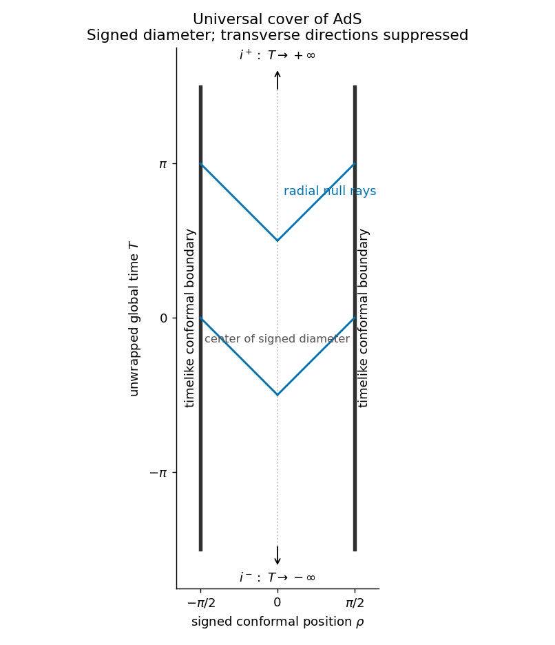
Conformal strip of the universal cover of anti-de Sitter spacetime, with timelike conformal boundaries and past/future timelike ends
. Details. 
The vertical edges are spatial infinity at every finite global time, forming the timelike boundary . The arrows mark the future and past timelike ends , conventionally and . There are no separate null-infinity edges like Minkowski : radial null rays satisfy and reach the timelike boundary in finite global time. Their physical affine parameter is nevertheless infinite there. The drawing is a finite excerpt of an infinitely tall strip, not an identification of its top and bottom. On the original hyperboloid global time is periodic and there are closed timelike curves; unwrapping it is essential to the usual physical maximally extended AdS spacetime.
A globally hyperbolic spacetime admits a Cauchy surface: every inextendible causal trajectory meets this spacelike initial-data surface exactly once. Physically, suitable field data on it determine evolution everywhere in its domain without additional data arriving from an unprescribed external boundary. This includes absence of causal loops and pathological almost-loops. An equivalent standard characterization is strong causality together with compact causal diamonds . The Cauchy condition concerns all causal curves, not merely the timelike geodesics that happen to remain in a bounded spatial region.
The universal cover of maximally extended AdS is not globally hyperbolic. Its timelike conformal boundary can send signals into the interior after any chosen initial slice, so bulk initial data alone do not determine evolution. In the conformal strip, a null ray can run from to the center in global time ; it need not meet a sufficiently earlier constant-time slice within the interior spacetime.
The compact-diamond test makes the obstruction explicit. Choose two central events with times and in units . Events at , lie between them causally, because their radial coordinate separation is less than2. They form a sequence in the causal diamond with no limit in the AdS interior. The diamond is therefore noncompact. Boundary conditions, such as reflecting conditions on the conformal boundary, can supply a well-posed initial-boundary-value problem; they do not turn the boundary-free interior into a globally hyperbolic spacetime in the usual definition. The periodic-time hyperboloid is also non-globally-hyperbolic, already because it has closed timelike curves.
In the ambient space of signature , AdS is . Let an arbitrary event have embedding vector , and let be any future unit timelike tangent, soThe complete family through that event isDirect substitution gives and . Its ambient acceleration is , normal to the hyperboloid, so its tangential covariant acceleration vanishes. This proves that is proper time and that each curve is a timelike geodesic, rather than just guessing sinusoidal tracks from the diagram.
An AdS isometry can place any chosen at . Rotate the spatial direction into the displayed signed diameter. Write the initial local velocity as , with . Then , and . Eliminating using the global coordinates givesVarying the speed gives the drawn family; suppressed spatial directions can be restored by varying the tangent direction. It represents all timelike initial directions after the isometry and spatial rotations.
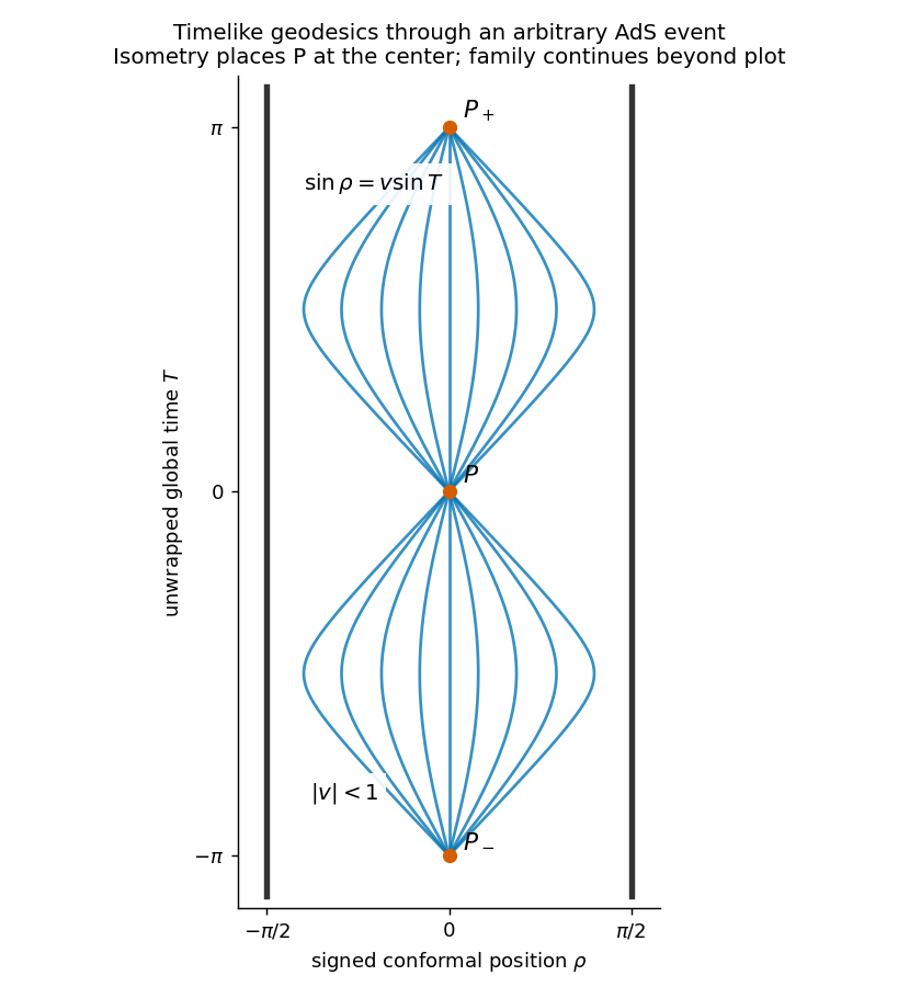
Timelike geodesics through an arbitrary AdS event, placed at the center by an isometry, refocusing at later antipodal events
. Details. 
Every finite-speed curve turns before the conformal boundary. At proper time , all reach ; at their ambient coordinates return to . This is Anti-de Sitter timelike geodesic refocusing. On the universal cover the global time has advanced by and , respectively, so these are later events. They are not closed timelike curves. The limits approach the null directions and are not timelike members of the family.
Set . The metric becomesso these are Poincare coordinates on anti-de Sitter spacetime with unit curvature radius. They cover one patch, not the whole global extension.
On the two-dimensional section with the three transverse suppressed, choose embedding coordinates , , . The Poincaré transformation isChoose the connected component containing . Its denominator is positive, givingIts two sloping edges are Poincaré horizons, null coordinate boundaries at . The right vertical edge is the timelike conformal boundary. Substituting the transformation into gives , verifying the chart and its null edges.
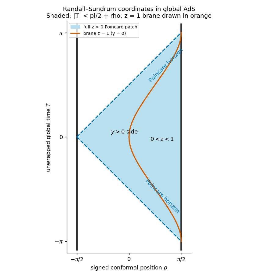
The Randall-Sundrum Poincaré patch inside global AdS, with null patch horizons and the reference brane z=1
. Details. 
The full coordinates in this part have , hence the whole shaded patch. If one additionally retains only the Randall–Sundrum bulk as in Question4, keep . The brane , or , has and is drawn in orange; the retained side contains , . A patch horizon is not a curvature singularity or the timelike conformal boundary. A geodesic can cross it in finite proper time while the patch coordinate diverges.
Use dots for derivatives with respect to proper time and the given unit curvature radius. Translation symmetry in the four brane coordinates gives constantsFor a future-directed timelike curve . The unit-tangent constraint isIt follows that and . Set . Thenwith solution on an interval where the cosine is positive. A phase shift includes either sign of the initial radial velocity. Integrating the four conserved-momentum equations gives the most general trajectory within this patch:The arbitrary constants encode the initial location and every unit timelike initial velocity. For the past-directed orientation reverse the tangent. The radial turning point is ; the two limits are patch horizons, not the endpoints of the complete globally extended geodesic. This is the timelike geodesics in a warped Poincaré patch solution. As a check, and , which are the explicit geodesic equations.
To measure the acceleration of the surface, take an observer at rest in its flat coordinates: there. The relevant Christoffel coefficient isThereforeIt points toward decreasing . More generally any observer moving inertially within the brane satisfies , and gives the same normal acceleration. The brane's extrinsic curvature for normal is , consistent with this result. Restoring curvature radius gives warped-brane proper acceleration . Intrinsically the induced brane metric is Minkowski and these observers have zero four-dimensional proper acceleration; the nonzero acceleration is relative to the bulk.
In the one-brane Randall–Sundrum model, gravity localization in a noncompact warped dimension produces a normalizable massless graviton despite the infinite proper fifth dimension. At long distances its zero mode reproduces four-dimensional gravity; bulk Kaluza-Klein modes give corrections. This localization mechanism, rather than a large compact volume, is the reason an infinite dimension need not destroy the usual Newton law, as established in the original single-brane warped-gravity construction. Its observational tests include:
- Short-distance gravity experiments. Massive bulk modes supplement the localized zero mode, changing the gravitational potential near the AdS curvature length. Torsion balances, microscopic force measurements and suitable precision gravitational tests can seek departures from the inverse-square law. The relevant scale is the warp curvature length, not a finite compactification radius.
- Collider missing energy. If the bulk gravitational scale and couplings are accessible, collisions can emit gravitons into the fifth dimension; a visible jet or photon recoils against unobserved energy. Virtual bulk modes can also change scattering rates and angular distributions. The minimal one-brane spectrum is a continuum, not the discrete resonant tower of a two-brane model, so those predictions must not be interchanged.
- Gravitational-radiation tests. Additional bulk propagation channels can modify energy loss, waveforms or propagation at sufficiently high frequencies. Binary timing and gravitational-wave measurements probe such departures. The localized low-energy mode makes four-dimensional propagation a good approximation; large long-distance leakage is not automatic.
- Astrophysical energy loss. Dense hot objects could radiate accessible bulk modes, changing cooling histories. Supernova and compact-star observations can limit such channels, with rates determined by the specific warped spectrum and coupling.
For an expanding brane, its motion in the bulk and the Israel junction conditions modify the four-dimensional cosmological expansion. In the tuned low-energy regime it approaches ordinary cosmology, but high-energy braneworld expansion has a density-squared correction when the matter density approaches the brane tension. Faster early expansion changes weak-interaction freeze-out and light-element yields, so Big Bang nucleosynthesis is a sensitive test. It also changes time-temperature relations, recombination distances and acoustic scales in the Cosmic microwave background anisotropy.
The bulk can supply dark radiation on a cosmological brane, a projected-Weyl contribution that scales like radiation and is related to a bulk black-hole mass in the simplest vacuum construction. Nucleosynthesis and CMB measurements constrain its contribution to the expansion. Energy transferred from a hot brane into bulk gravitons can further modify the radiation history. None of these terms must be identified with an ordinary thermal particle component without a model.
Inflation on the brane can alter scalar and tensor production at high energy; the gravitational-wave zero-mode normalization and coupling to bulk modes can change primordial spectra. CMB temperature/polarization, primordial gravitational waves and later structure growth can test these effects. Projected bulk perturbations may introduce nonlocal corrections to the brane's effective perturbation equations, so a background expansion law alone does not determine all observables. Late-time measurements of expansion and structure also test residual departures, although the basic tuned model does not automatically predict dark-energy acceleration.
All proposed signals depend on the curvature scale, fundamental gravitational scale, brane tension, reheating history and bulk state. The minimal single-brane construction has no second-brane separation radion; an arbitrary radion fifth-force prediction from a two-brane compactification cannot simply be imported here. The main probes are corrected gravity, accessible bulk radiation, and high-energy/dark-radiation changes to cosmological evolution.
For flat compact large extra dimensions, gravity spreads through all spatial dimensions at distances smaller than the torus size, while ordinary Standard Model matter remains localized on the brane. At distances much larger than , only the massless gravitational zero mode is important and ordinary four-dimensional gravity is recovered. The large compact volume weakens the observed gravitational coupling, allowing a lower fundamental bulk scale. The extra modes have momentum quantized around the circles and appear on the brane as a dense Kaluza-Klein tower with mass spacing of order .
Distinct experimental and observational probes are:
- Short-distance force laws. Below , gravitational flux explores the extra dimensions, so the force falls faster than the ordinary inverse-square law. Precision torsion balances and microscopic-force experiments can seek the crossover and constrain the size and number of dimensions. Electromagnetic surface forces must be separated from the gravitational signal.
- Real graviton production. At energies resolving the extra dimensions, many KK final states become kinematically accessible. Their multiplicity can compensate for each mode's weak individual coupling, producing missing-energy events with a jet, photon or other visible recoil at colliders. Ordinary invisible particles are backgrounds, so energy and angular distributions and consistency between channels matter.
- Virtual KK exchange. The tower can alter dilepton, diphoton and other scattering distributions through extra spin-two exchange. Its energy and angular dependence provides complementary information to missing energy. Predictions approaching the fundamental scale depend on the ultraviolet completion rather than on low-energy effective theory alone.
- Stellar and supernova cooling. Gravitational modes emitted from hot dense matter carry energy out of the observed brane sector. Cooling times and supernova neutrino observations therefore constrain accessible KK populations. Trapped modes or modes produced earlier can also decay later and heat compact stars.
- Decay radiation and cosmological abundance. Massive KK gravitons can have long lifetimes; their decays can create diffuse gamma rays or other radiation. Excess early production can overclose the universe, disturb nucleosynthesis, alter the CMB spectrum, or inject energy after recombination. These tests depend strongly on reheating temperature, mode lifetimes and decay channels.
- Radius dynamics. Compactification requires a mechanism stabilizing the torus radii and shape moduli. A light radion or other modulus can mediate an extra force, violate the expected universality of free fall through its couplings, or vary effective gravitational/particle constants. Precision force tests, atomic clocks and astronomical comparisons can constrain those effects. They are conditional on the modulus being light and sufficiently coupled; stabilized heavy moduli can evade them.
- High-energy gravitational phenomena. If the fundamental bulk scale is sufficiently low, scattering may reveal strong gravity or microscopic black-hole-like states. These are possible ultraviolet signals, not robust predictions at arbitrary accessible collider energy. Bulk-mode channels can also affect sufficiently short-scale gravitational radiation.
The size and number of extra dimensions enter both the force-law crossover and KK state counting, enabling consistency tests between these probes. Existing four-dimensional agreement does not by itself exclude a sufficiently small or weakly accessible compactification. Conversely a single generic missing-energy anomaly is not a unique signature: it must agree with the tower and gravitational interpretation across observations. Compact flat models are chiefly tested through the radius-dependent gravitational crossover, KK production/exchange, and the thermal/cosmological fate of bulk modes, with radius-stabilization effects as an additional model-dependent channel.
Articles by others on the same topic
There are currently no matching articles.