Take to be linear in its first argument and conjugate-linear in its second, with . For a Hermitian form over a quadratic finite field, . We first establish the quadratic finite-field norm and trace surjectivity needed for orthonormalization of a finite-field Hermitian form. The field norm maps onto because the multiplicative group of a finite field is cyclic of order . The field trace is an -linear map into . It is nonzero: a nonzero polynomial of degree cannot vanish at all elements. It is therefore onto, including in characteristic two.
There must be with . Otherwise, for any , expanding the diagonal value givesIf , varying contradicts the surjectivity of the field trace. Thus all pairings would vanish, contrary to nondegeneracy. Choose with ; then has norm one. Every decomposes uniquely asThe restricted Hermitian form over a quadratic finite field on the orthogonal complement for a sesquilinear form is nondegenerate: a vector there orthogonal to that complement is also orthogonal to , hence to all of , and is zero. Induction produces an orthonormal basis .
The unitary group over a finite field is the group of invertible -linear maps preserving . In the orthonormal basis just constructed, its concise description isThe notation here uses the size of the matrix field; it is also frequently written . There is no determinant-one condition in this definition.
We construct a Hermitian hyperbolic plane over a finite field inside each successive two-dimensional piece. By the field norm surjectivity proved above, choose with . From two vectors in an orthonormal basis, form . Then , so is a nonzero isotropic vector. Nondegeneracy supplies with ; rescaling the second argument achieves this normalization. In fact already works in this two-dimensional piece. By quadratic finite-field norm and trace surjectivity, choose with and put . Direct expansion givesThus are linearly independent, and their Gram matrix is , which is invertible even in characteristic two. Their span is nondegenerate, so its orthogonal complement for a sesquilinear form is again nondegenerate. Repeat the construction there. In even dimension this exhausts ; in odd dimension the final one-dimensional complement has a nonzero diagonal value, which can be normalized to one using the field norm. Calling its vector , we obtainwith the terms present only in odd dimension. This proves all the requested pairings and the basis assertion.
The printed hint needs a qualification. If is irreducible over , its two roots are conjugate, so and ; the hinted vectors then do work. They need not work when it splits. For example, over its roots are , fixed by conjugation in . For either choice the proposed has norm , respectively or , rather than zero. The norm-and-trace construction above proves the assertion without that restriction.
Use the course convention that a root system is finite and is a reduced root system satisfying the crystallographic root system condition. These hypotheses are essential for the angle restriction. For roots , the two Cartan integerssatisfy . If are not parallel, the strict Cauchy-Schwarz inequality and integrality give . These values give angles , or , or , and or , respectively. If the roots are parallel, reducedness implies , giving or . ThereforeHere are examples accounting for every angle. In the A1 root system, the pairs and give . Two roots from different summands of give . The six unit vectors at angles form an A2 root system: taking one root at angle zero and another at or gives those two angles. In the B2 root system , pair with or to obtain . In a G2 root system, take short unit roots at angles and long roots of length at angles . A short root at zero paired with long roots at gives the remaining angles.
If the roots are parallel, their Euclidean norms are equal by reducedness. For nonparallel, nonorthogonal roots, the Cartan integers above are nonzero integers of the same sign and have product or . AlsoThe absolute pairs are , , or . HenceMore precisely, angles require equal lengths; angles require a long-to-short ratio ; and angles require a ratio . The exclusion of orthogonality matters: orthogonal irreducible components can be scaled independently.
Choose a fundamental system of a root system . Distinct simple roots have nonpositive inner product. Their Cartan matrix has diagonal entries two and off-diagonal entries , where either , or are positive integers. The root-system finiteness lemma gives . After exchanging the simple roots, the possibilities areTheir angles and relative lengths determine the two simple roots up to an orthogonal transformation and common scaling, except that the two orthogonal components can be scaled separately.
To see that no extra roots remain unspecified, write a positive root with nonnegative integer coefficients. If it is not simple, some simple root has : otherwise . The root reflection in subtracts a positive integer multiple of . The other coordinate stays nonnegative; since is not proportional to , it is positive, so the reflected root must still be positive by the defining sign property of a fundamental system of a root system. Its height decreases. Repeating reduces to a simple root. Thus every root is in a Weyl group orbit of a simple root.
For the four matrices, applying their simple reflections gives, respectively, the following positive roots:where in the last two rows is long, short. For example, and for the displayed matrices when the convention is . The sets comprising these positive roots and their negatives are invariant under both reflections, as direct substitution verifies. The height argument therefore shows they are the whole root system. This proves the classification of rank-two root systems:
A Dynkin diagram has one vertex for each simple root. Vertices are joined by bonds, where are the off-diagonal Cartan integers. No bond means orthogonality; one, two and three bonds mean angles . A multiple-bond arrow points to the shorter root. Thus the Dynkin diagram determines the Cartan matrix, including the relative lengths inside each connected component.
An irreducible root system corresponds to a connected Dynkin diagram. The classification of finite crystallographic Dynkin diagrams givesHere is already represented by , and by . General systems are orthogonal direct sums of these, with separate component scales. The following diagrams specify all the types; dots denote a continued chain, not additional vertices.
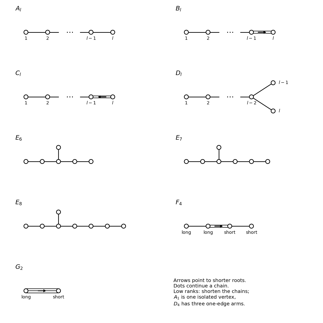
Finite irreducible crystallographic Dynkin diagrams, with every arrow pointing toward the shorter root
. Details. 
For orientation, the An Dynkin diagram is a single chain, the Bn Dynkin diagram has a terminal double bond pointing to its terminal short root, and the Cn Dynkin diagram reverses that arrow. The Dn Dynkin diagram has arm lengths . The En Dynkin diagram has arm lengths ; ; or . The F4 Dynkin diagram has a central double bond and the G2 Dynkin diagram a triple bond.
The positivity behind this finite list is the positive-definite Gram matrix of the simple roots. In particular the underlying graph is a tree: if it contained a cycle, the sum of its normalized roots would have squared norm at most zero, since each bonded inner product is at most . This contradicts linear independence. Restricting the possible bonds and branches by positive definiteness gives precisely the listed chains and trees. Conversely their Cartan matrices are positive definite after symmetrization and their reflection-generated root sets give the indicated finite root systems.
Put and . These elementary matrices belong to the special linear group. Let have determinant one. If , elementary row elimination givesThe remaining diagonal matrix is also a product of the given generators. Indeed, for , direct multiplication givesHence . If , its determinant forces , and has upper-left entry . The established case applies to it, and is again generated. No division by two was used, so the proof works over every field. The upper and lower elementary unipotent matrices generate .
Here denotes the adjoint Chevalley group of type A1; the isogeny form matters, since the simply connected form is itself. Over , take the sl2 Lie algebra with Chevalley basisTheir Lie brackets satisfy , , . Conjugation defines a group homomorphism . Since , and . Differentiating conjugation, or expanding its finite polynomial on this basis, givesThe adjoint Chevalley group is generated by these two families. Part (i) therefore proves that it is exactly the image of . A matrix commuting with has the form ; also commuting with forces . Thus the kernel of a group homomorphism consists of scalar matrices of determinant one, namely . The first isomorphism theorem now gives .
For a general field, first compute the Chevalley basis root operators as integral polynomials, and only then reduce their coefficients to . Explicitly,They are still precisely conjugation by on the three-dimensional trace-zero matrix space. These formulas remain valid in characteristic two, where but remain linearly independent. Part (i) still identifies the generated image with the conjugation image of . The same computation with gives kernel of a group homomorphism , exactly its scalar center. ConsequentlyIn characteristic two the scalar center is trivial. The integral formulas avoid the invalid operation of dividing by factorials inside a field of small positive characteristic.
The Lie bracket is bilinear, so is a linear map. Rearranging the Jacobi identity givesThuswhich is the defining Leibniz rule for a derivation of a Lie algebra. In particular is an inner derivation of a Lie algebra.
Write , and choose with . The exponential of a nilpotent Lie algebra derivation is the finite linear operatorFor a derivation of a Lie algebra, induction on using the Leibniz rule and Pascal's identity provesExpanding and grouping by consequently givesTerms with an exponent at least vanish, which justifies extending each inner sum; and for . Finally the finite product of the two exponentials has coefficientso is the inverse. We have proved bracket preservation and invertibility, hence is a Lie algebra automorphism.
Because is a Lie algebra automorphism, for every ,Conjugation therefore also proves that is a nilpotent operator, and sends every power of to the corresponding power of . Applying this to the defining finite exponential of a nilpotent Lie algebra derivation yields
Apply the Jacobi identity to an arbitrary :Thus the Adjoint representation of a Lie algebra preserves the Lie bracket:
The root-space decomposition gives when . The two roots are independent, so , and the missing root sum means that this weight space is zero. Hence . These adjoint root operators are nilpotent: successive brackets shift root weights by the same root, so finite root strings force eventual vanishing; on the Cartan subalgebra the first bracket lies in its root space and the next is zero. By part (iv), the nilpotent operators and commute. Every power of therefore commutes with every power of , so their finite matrix exponentials commute too. Using the inverses proved in part (ii),
Let every root have squared length . Since is a root, , hence . In particular the roots are independent. The potential higher sums satisfyso neither is a root. The root-space decomposition therefore gives .
Set , and . Part (iv) shows . To compute the sign, differentiate :Thus . Conjugating the matrix exponential, and then using the commutation of , givesThis proves the central-commutator exponential identity in the required order, and consequently the simply laced Chevalley commutator formula is
The map is linear, so its kernel is a vector subspace of the matrix algebra. If , use to computeThus is closed under the commutator. This bracket is bilinear and satisfies . Associativity of matrix multiplication gives the Jacobi identity: expanding makes each of the six ordered triple products occur once with each sign. Therefore is a Lie algebra. No nonsingularity or symmetry assumption on was needed.
For the nilpotent matrix , define the polynomial . Because , differentiating gives . The derivative of the preserved bilinear form matrix is thereforeIt is a constant matrix polynomial, equal to at . Evaluation at one provesAlso is the inverse of by the finite exponential product identity, so this really is an invertible isometry, even when is degenerate.
Write and . Block multiplication givesIts vanishing is equivalent toThis identifies with the symplectic Lie algebra .
We now supply the requested root-space decomposition, including explicit vectors. Let be the matrix units, put , and define the linear functionals on the diagonal Cartan subalgebra by . Then . The Cn root system and a corresponding matrix root basis of the symplectic Lie algebra areEach listed vector satisfies the block conditions just proved. For a diagonal matrix , the matrix unit calculation gives all the requested eigenvalues explicitly:The diagonal vectors and difference-root vectors span every possible block. The sum-root and doubled-root vectors span all symmetric and blocks. They are linearly independent, as is evident from their disjoint independent block entries. Equivalently there are of them, exactly the dimension of . The zero weight space is precisely : a zero weight forces diagonal and every entry of to vanish. Hence every nonzero root space is one-dimensional and
Articles by others on the same topic
There are currently no matching articles.