Each operator has trace one, so its characteristic polynomial is . The first and last are diagonal; for the others, the symmetric and antisymmetric vectors diagonalize the matrix. Their eigenvalues areFor , has eigenvalue one and has eigenvalue zero. For , those eigenvalues are and , respectively. All four density operators are positive semidefinite, as these spectra confirm.
A density operator represents a pure state exactly when it has rank one, equivalently or . The spectra just found giveTheir wavefunctions are defined up to a global phase. The other two are mixed states, with purity , and have no single-wavefunction representation as rank-one projectors.
Two finite-dimensional Hermitian matrices are related by unitary conjugation if and only if they have the same multiset of eigenvalues. Necessity follows because conjugation preserves the characteristic polynomial; sufficiency follows by mapping orthonormal eigenbases in the spectral theorem. Consequentlyand no member of the first pair is equivalent to a member of the second. For an explicit example, the Hadamard gate gives and . Multiplying by a scalar phase does not change either conjugation.
The Von Neumann equation integrates to , so the spectrum and purity of a density operator are invariant under any allowed open-loop control. These are the kinematic restrictions.
There is no additional orbit restriction here: the generators and , together with their matrix commutator, span the special unitary Lie algebra:For freely chosen durations and piecewise continuous real control values, this gives density operator controllability. The connected reachable group is ; its action by conjugation is the same as that of , because a global phase cancels. Thus exactly the pairs and can be interconverted. No coherent control can turn either mixed state into either pure state, even though every orientation within each spectral orbit is reachable.
Here “controllable” means density operator controllability, so all transformations on a fixed spectral orbit are available. Strict unitary operator controllability, including an independently specified global phase, is a stronger condition. Assume the usual finite-dimensional real controls and freely chosen duration.
The dimension hypothesis actually identifies the algebra, not just its size. For completeness, put the invariant inner product on and write . Since is closed under commutators, lies in for every . The adjoint action is skew-adjoint for this inner product, so is also orthogonal to and must vanish. If were nonscalar, its orthogonal eigenspaces would give a centralizer of dimension at most , too small to contain . Therefore is scalar and . This proves codimension-one quantum dynamical algebra is special unitary.
a1 is true for density-state controllability; a2 is true; a3 is false. The algebra generates every determinant-one unitary. For any , choose with ; then , proving that every gate is available up to global phase. But all generated Quantum Hamiltonians are traceless, andso evolution starting at the identity always has determinant one. Arbitrary determinant, requiring the additional central direction , cannot be generated. If a1 is instead read as phase-sensitive unitary-operator controllability, it is false for precisely the same reason as a3; the physical distinction is explicit here.
The stated relation places every generator, and therefore the whole Dynamical Lie algebra, inside the standard compact symplectic Lie algebra . Indeed the relation is closed under linear combinations and commutators, and differentiating evolution givesThus it supplies a symplectic dynamical symmetry in quantum control, rather than a claim that commutes with every Quantum Hamiltonian.
For , b1 is false: even the full compact symplectic group does not act transitively on every mixed-state spectral orbit. Its algebra has dimension . An explicit obstruction is the symplectic invariant of a density operatorwhich is unchanged by a symplectic conjugation. For and the printed , let , , . The isospectral operators and have invariants and , respectively, and cannot be interconverted. For the exceptional case , , so b1 cannot be decided from inclusion alone; equality gives density-state controllability.
b2 is not implied by the displayed relation: more information is needed. It permits the full symplectic algebra but also a single commuting generator, or even zero generators. The full is pure-state controllable: identify with , extend any unit vector to a quaternionic orthonormal basis, and map one such basis to another. A one-axis diagonal subgroup, in contrast, cannot change level populations.
The required extra information is the generated algebra, obtained by computing its real span of iterated commutators. Within this specified symplectic inclusion, equality gives pure-state controllability; its dimension is . The mere inclusion does not establish equality. For , equality also answers b1 affirmatively. None of these strictly symplectic generators supplies arbitrary global phase.
c1 is true for density-state controllability. Every qubit density operator can be written using its eigenvalues. A control taking one pure orthogonal projector to any other therefore also connects every pair of qubit density operators with the same spectrum. In Lie-algebra language, ; there is no larger-dimensional symplectic exception. This does not supply arbitrary global phase: alone is already a counterexample to an implication involving strict operator controllability.
c2 is false. For every even , the defining action is transitive on unit vectors, so a system generating this algebra is pure-state controllable. It still preserves additional mixed-state invariants and lacks density operator controllability, as the preceding explicit four-dimensional example demonstrates. pure states have fewer orbit requirements than general mixed states.
True for the finite bound-level Morse model with nonzero adjacent control couplings. The Morse oscillator energies have the formOver the physical bound-level range these adjacent gaps are positive, and makes them pairwise distinct. Label the retained levels consecutively. With , all , the squared adjoint action of has eigenvalue on each adjacent skew-Hermitian coupling. A polynomial chosen by Lagrange interpolation can therefore isolate any one adjacent coupling from .
Commuting an isolated coupling once with the drift produces its independent antisymmetric quadrature. The bracket between the two quadratures yields a traceless diagonal generator; brackets along the connected chain produce every nonadjacent off-diagonal generator. Thus connected nondegenerate transition chain generates special unitary control proves , which gives density-state controllability. If the physical drift has nonzero trace, subtracting its traceless part also produces the identity direction, giving and full operator controllability. Shifting the energy origin may remove that extra phase direction but does not change state controllability. The assertion concerns the finite-level model in the question, not the entire bound-plus-dissociation Hilbert space of the untruncated Morse potential.
Take the drift propagator with the correct initial normalization, , and define the interaction picture by . Differentiate this product and substitute the Schrödinger equation:Since , the drift terms cancel. Left multiplication by givesThe printed is this expression with time origin . Its differential identity remains valid at arbitrary , but its interaction-picture initial operator would then be rather than the identity. Using resolves that normalization without changing the derivation.
Use as in the displayed carrier-phase convention. The drift is diagonal, and conjugation givesMultiplying by and expanding the cosine into exponentials yieldsThe rotating-wave approximation averages away the components oscillating at , retainingThe envelope is slowly varying and the effective coupling is weak compared with the carrier frequency. The pulse phase selects the transverse rotation axis on the Bloch sphere; its pulse area determines the angle. Counter-rotating corrections are neglected under this approximation, not identically zero.
The original Figure 1 has the allowed chain . Its positive resonance frequencies are , and in units ; level 2 lies above level 3. Use a pulse at to transfer level population from 1 to 2, then one at to transfer it from 2 to 3, and finally one at to transfer it from 3 to 4.
For a selected pair, choose the optical phase so the effective Quantum Hamiltonian has a fixed off-diagonal rotation axis. If its coupling coefficient is in this normalization, the active two-dimensional propagator iswhere . A full level population transfer has . Equivalently, in the Rabi-frequency convention , the required area is . On spectator levels the embedded two-level quantum rotation is the identity.
Thus three selective pulses at , in that order, transfer to up to global phase. A strongly regular quantum Hamiltonian separates the resonances; envelopes long enough that their bandwidth and coupling strength are small relative to unwanted frequency gaps make off-resonant excitation arbitrarily small within the selective-pulse limit. The phases accumulated along this path do not affect the final level population.
Use geometric quantum state synthesis by adjacent rotations, rather than three full level population swaps. Each resonant pulse implements a complex Givens rotation on one allowed two-state plane. Start with the target amplitude vector, use such rotations to eliminate entries back to the first basis vector, and reverse that sequence. Its angles are fixed by the ratios of target amplitudes, and optical phases supply their relative complex phases.
Here is an explicit real-coordinate construction in the interaction picture. Define a phase-calibrated rotation byA resonant Quantum Hamiltonian proportional to realizes this rotation; the optical phase chooses that quadrature. Let . ThenThe pulse areas equal these rotation parameters in the direct Hamiltonian-coefficient convention of quantum pulse area. A given sign or phase choice for a physical transition depends on its dipole and basis conventions; calibration realizes the specified rotation without assuming every adjacent transition has the same energy ordering.
If the requested amplitudes refer to the laboratory frame at , the target for this construction is , not simply . Set the rotation phases accordingly, or add the equivalent accessible diagonal phase corrections. This compensates the known drift phases and gives the stated laboratory superposition, not merely the correct level populations. Strong regularity and connected allowed transitions guarantee the required controllability; bandwidth restrictions set how slowly the selective approximation must be implemented.
The terminal term is the objective reward. With the Hilbert-Schmidt inner product , a Hermitian target observable gives its final expected value. The vector is the density operator represented as a vector in operator space; it retains the same physical content as the density matrix, not a wavefunction of the system.
The term imposes the dynamical equation by a time-dependent costate . It is a Lagrange-multiplier operator in the same operator space, propagated backward from a terminal condition. It is not required to be a positive, trace-one density matrix. DefineThen the enforced state equation is . The uncontrolled coherent part is , the dissipative contribution is , and each describes a control coupling. For Quantum Hamiltonian control, .
The term is a quadratic field-energy or fluence penalty. For the positive scale and positive weights , larger make a given control amplitude more costly. Thus maximizing trades terminal performance against control fluence while enforcing the dynamics. The multiplier term vanishes on any dynamically feasible trajectory. The weights do not represent decoherence rates; they specify control-resource preferences.
At an unconstrained differentiable extremum the first variation vanishes independently with respect to the state, costate and real controls, with initial state fixed. For the real functional, take the real Hilbert-Schmidt pairing when necessary. The Euler-Lagrange equations are most clearly written using the forward generator :Here the dagger is the adjoint for the Hilbert-Schmidt inner product, and is the vectorized terminal observable. Equivalently,The adjoint is essential if is not self-adjoint: dissipative costate evolution must not be replaced by the forward dissipator.
For each unconstrained real field, stationarity givesThus . For Hermitian state and costate with Quantum Hamiltonian couplings, the contraction before taking its imaginary part is purely imaginary, and this is a real field. These are the Liouville-space costate equations for quantum optimal control.
Forward state propagation, backward costate propagation, and the control stationarity equations must be solved together. They give necessary conditions, not a certificate of global optimality. For a local maximum the second variation on admissible perturbations is nonpositive. If amplitude or bandwidth constraints are imposed, the unrestricted pointwise field equation must be replaced by the corresponding constrained stationarity condition.
For the first two targets assume , so the indexed levels exist. A possible level population reward isIt selects and .
For the coherent target, use its rank-one orthogonal projector, not the sum of its two level populations:The imaginary quantum coherence term fixes the desired relative phase . Maximizing level populations alone would not select this superposition.
For energy, choose a specified final energy observable :For stored energy after the control is switched off, is the natural choice. If a fixed external field remains, use that known final Quantum Hamiltonian instead. If the terminal Quantum Hamiltonian itself is varied through the controls, the objective has explicit control dependence and additional terminal derivatives must be included. Each reward can be combined with the given dynamics and fluence penalty as .
Use spectral pulse shaping of a broadband coherent laser pulse. A 4f pulse shaper disperses the frequency components with a diffraction grating, maps them to different transverse positions with a lens, applies a programmable complex mask at the Fourier plane, and recombines them with a second lens and grating. A spatial light modulator or suitable amplitude-and-phase modulation stages impose the mask.
Compute the desired complex spectral field by Fourier transform of the required temporal envelope, including its phase. In the available spectral band, chooseThe mask amplitude changes the spectral weights, and its phase changes temporal interference and chirp. Recombining the masked spectrum produces the shaped temporal pulse. A phase-only device needs additional optics to implement independent amplitude control. Calibrate the mask-to-frequency mapping and verify the output pulse experimentally, correcting it iteratively if needed.
The source bandwidth must contain the requested spectral components; a passive mask attenuates rather than supplies missing energy, so an overall rescaling may be needed. Finite spectral resolution determines the accessible time window, and finite bandwidth limits rapid temporal features.
Work with real positive pulse envelopes and define . Then and . In the ordered basis , the candidate dark state of a driven Hamiltonian has coordinatesMultiplication by the given rotating-wave approximation matrix givesThusIts absence of an excited-state component is the destructive interference that makes it dark. The orthogonal bright ground-state combination is . Since and , the two remaining eigenstates are with eigenvalues .
For signed envelopes, use a continuous two-argument angle with and , rather than an ambiguous arctangent branch. When both fields vanish, every state has zero eigenvalue and this formula does not select a unique dark vector.
Start by turning on first, while . The dark state is then exactly , which is uncoupled even while the first pulse rises. Next turn on while remains appreciable, and then turn off while remains on. The ratio rises from zero to infinity, soThe final minus sign is an irrelevant global phase for level population transfer. This is the counter-intuitive sequence of stimulated Raman adiabatic passage: the laser coupling the target state to the excited state precedes the laser coupling the initial state to the excited state.
The quantum adiabatic theorem requires the dark state to rotate slowly compared with its separation from the bright states. Here , so its coupling to either bright eigenstate has magnitude . In the printed convention the entries are angular-frequency couplings, and the condition isIf one instead uses an energy-valued Quantum Hamiltonian, its spectral gap is and the same condition is . Maintain nonzero overlap and gap while the angle changes. The pulses can vanish at the beginning and end, where the dark state has stopped rotating and is an exactly decoupled basis state.
An explicit smooth sequence has on and zero otherwise, while on and zero otherwise. Choose . The first pulse comes earlier, both overlap during the rotation, and the second persists after the first has ended. The following original sketch shows the envelopes and instantaneous dark-state level populations.
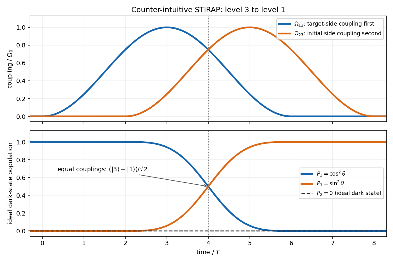
Counter-intuitive STIRAP pulses for transfer from level 3 to level 1, with ideal dark-state populations
. Details. 
Excited-state decay is suppressed in the ideal dark-state limit. The dark state has zero amplitude on , so a spontaneous-emission jump of the form annihilates it. There is consequently no excited-state level population to decay in perfect adiabatic following. Finite speed introduces bright-state admixture and a small excited level population; its integrated loss is of order . Thus robustness is conditional on good adiabaticity, not immunity to arbitrarily large decay at fixed pulse strength and duration. In a strongly overdamped regime the relevant relaxation gap can also limit following.
Moderate envelope perturbations are tolerated because this transfer is fixed by the endpoints of the dark-state path, not by an accurately calibrated resonant pulse area. Common amplitude changes do not change the angle, although reducing them too far closes the useful gap. Independent smooth changes still work if they preserve the counter-intuitive order, the endpoint ratios, resonance and a sufficiently large gap relative to . A wrong sequence, missing overlap, rapid fluctuations or unstable relative optical phase can spoil the transfer.
Ground-state decoherence is not suppressed by the dark-state mechanism. During the overlap, the dark orthogonal projector has quantum coherence . Dephasing of the – transition removes precisely this relative-phase information, even if initially. For example, with in a Lindblad equation, its dissipator gives . It therefore drives a nontrivial dark superposition away from its pure orthogonal projector. The transfer should be slow enough for adiabaticity but fast compared with the relevant ground-state quantum coherence lifetime. Ideal protection from excited-state spontaneous emission does not protect this ground-state quantum coherence.
With the principal arctangent in part (a), both coefficients must be . HenceFor the positive-envelope transfer this is the crossing at a positive coupling. If both couplings have the same negative sign, their ratio still gives the stated principal-angle vector; a continuous-angle representative can differ by an irrelevant overall minus sign. At this point the instantaneous dark state is . In the example sketch this occurs at , where the two effective couplings cross. Equality of the raw envelopes and is not enough if the dipole moments differ: the condition is , with the same effective relative phase. More generally the equality may occur once or several times, depending on the pulse shapes. Simultaneous zero couplings do not specify this superposition because the whole Quantum Hamiltonian is then degenerate.
Articles by others on the same topic
There are currently no matching articles.