Work in geometrized units , with the stationary Killing vector field normalized by at infinity. Put , , and ; is the areal radius. The static spherical Komar mass in reciprocal radial gauge givesIndeed the future and outward unit normals to a round sphere are and , and . The Komar mass integral is therefore . Since and ,Taking the asymptotic limit yieldsThis agrees with . The finite-radius Komar integral need not equal its asymptotic value, because this solution is not vacuum. Restoring divides the mass expression by when has dimensions of length.
For radial null geodesics, the radial metric is . Define the tortoise coordinate byThen the radial metric becomes . Its two null directions have , so in the exterior. The radial null curves are null geodesics up to reparametrization: in the two-dimensional radial metric a null tangent's acceleration is proportional to itself, and spherical symmetry introduces no angular acceleration.
Since , the inverse- radial terms cancel. The ingoing Eddington-Finkelstein coordinates giveAt , . Thus all coefficients are analytic there, and the determinant of the metric block is , not zero. The angular area is also nonzero. This is an analytic extension of a spacetime through the apparent coordinate singularity, into the regular region .
For an asymptotically flat spacetime with future null infinity , its black-hole region iswhere the causal past is understood in the conformal completion. Choose the future orientation in the advanced chart so that is future null. For any future causal tangent , the inequality gives . The causality inequality isIf , it implies . Inside , , so strictly decreases. If , the angular tangent vanishes and future orientation makes a positive multiple of , again decreasing . Thus no future causal curve from can reach the exterior or future null infinity: it is inside the black-hole region.
Conversely, from any point with , the outgoing radial null geodesic has constant and . It continues to arbitrarily large , with , and reaches the corresponding future null infinity. Hence in this advanced exterior chart. This argument concerns the black-hole interior covered by ingoing coordinates; the additional white-hole region of the maximal extension has a different future causal orientation.
In advanced coordinates, is a Killing vector field and . The normal covector to is ; raising it gives , which equals on the horizon. Thus is a null hypersurface normal to , and hence a Killing horizon.
The surface gravity is defined by on this horizon, equivalently . Here , so the radial component gives . Because ,It is positive for all finite real and ; the stationary Killing vector field retains its asymptotic normalization.
Set . Since , the integrand defining the tortoise coordinate has a simple pole:where is analytic near . Define the Kruskal–Szekeres coordinates in the right exterior by and . ThenThe right-hand side has positive nonzero derivative at . Continuing this relation analytically, rather than retaining an absolute value, makes an analytic function of through both signs. The Kruskal extension across a simple static horizon has metricIts radial coefficient tends to , finite and nonzero, while . Therefore both null surfaces and are regular horizon branches, intersecting at a smooth two-sphere .
The stationary Killing vector field becomesIt is null, tangent and normal on each horizon branch and vanishes on their intersection. This proves that is a bifurcate Killing horizon, with bifurcation surface of area . The exponential definitions specify one exterior; allowing all signs of supplies the remaining quadrants of the extension.
There is only one zero of , at , and the Kruskal–Szekeres coordinates give four quadrants. Both exterior quadrants have , while the future and past interior quadrants have . The tortoise coordinate is finite at : for , , and for it is . Throughout each interior , so constant- hypersurfaces are spacelike. The assumed curvature singularity at therefore forms a spacelike future boundary in the black-hole region and a spacelike past boundary in the white-hole region. At infinity, and , giving two standard asymptotically flat ends.
The resulting Penrose diagram is the same four-region causal diagram as the maximal Schwarzschild spacetime:
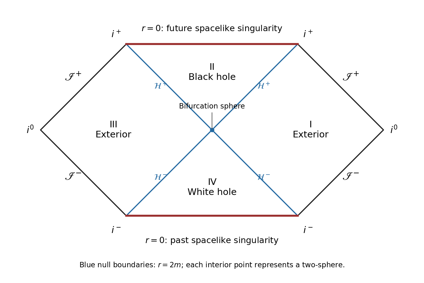
Maximal extension of the charged single-horizon geometry, with two exteriors, a black hole, a white hole and spacelike singularities
. Details. 
Each exterior has its own past null infinity, future null infinity, spatial infinity and timelike infinities. The future and past event horizons intersect on the bifurcation surface. The diagram describes the eternal analytic solution; a spacetime formed by collapse need not contain its white-hole region or second exterior.
Unlike a nonextreme Reissner-Nordstrom black hole, this electrically charged solution has one horizon and spacelike singularities, with no inner Cauchy horizon. A nonextreme Reissner-Nordstrom solution has two distinct horizons, including an inner Cauchy horizon, and a timelike singularity; its ideal maximal extension contains an infinite sequence of exterior and interior blocks. Charge by itself does not determine this causal structure: the metric and field equations of the gravitational theory matter.
An asymptotically flat spacetime is a stationary spacetime if it admits a complete stationary Killing vector field , with , timelike near infinity and normalized there to a unit time translation. It need not remain timelike in an ergoregion of a stationary spacetime. It is axisymmetric if it admits an axial Killing vector field , whose flow is a rotational action: its spacelike orbits away from the axis are closed with period , and it vanishes on the regular rotation axis. For a stationary axisymmetric spacetime, the generators can be chosen to commute, . These are geometric symmetries, not merely time-independent or angle-independent coordinate labels.
During gravitational collapse, nonspherical time-dependent multipoles can be lost in gravitational radiation or absorbed by the forming black hole. Matter remaining outside must ultimately escape or fall in if the final object is to be an isolated vacuum black hole. Assume that the classical exterior settles to a regular stationary asymptotically flat vacuum geometry, with a connected horizon and the regularity conditions of the black-hole uniqueness theorem. This settling assumption is physical input, rather than a consequence of charge conservation alone.
For a rotating remnant, the black-hole rigidity theorem supplies axial symmetry; the uniqueness theorem then identifies the exterior as Kerr spacetime. The nonrotating equilibrium case is Schwarzschild spacetime. Gravitational radiation carries energy and angular momentum but no net electric charge. In the intended neutral collapse, with no net charge carried away by expelled matter, charge conservation therefore leaves zero black-hole charge. Initial total neutrality alone would not prove this if oppositely charged matter were expelled; the two-parameter conclusion assumes the uncharged vacuum remnant just described. This leavesas its two intrinsic continuous parameters. The final are what remain after escaping matter and radiation have carried off their shares; they need not equal the star's initial values. A spatial rotation may align the spin axis, and a translation or boost chooses the position and rest frame, so these do not add intrinsic parameters. All higher equilibrium multipoles are fixed by ; for example Kerr's mass quadrupole is . A regular Kerr black hole obeys in geometrized units. This is the content of the black-hole no-hair theorem in vacuum general relativity, with its stated hypotheses, rather than a statement about arbitrary matter theories or an unproved guarantee of dynamical settling. Hawking evaporation is ignored in this classical late-time equilibrium description.
The conserved Killing energy of a geodesic tangent is , where . Conservation follows from and the Killing equation. For the Kerr metric, . Outside the outer Kerr ergoregion, is timelike. Its orthogonal complement is positive definite, so a nonzero causal vector cannot have . Equivalently, if both are future-directed, . HenceThis excludes the open exterior of the stationary-limit surface; on the surface itself a zero-energy null tangent can be proportional to the null stationary vector.
A Killing horizon must be a null hypersurface whose normal is a Killing vector field. The outer stationary-limit surface instead has and, in Boyer-Lindquist coordinates,On it, , so away from the rotation axis. Its normal is spacelike and the surface timelike. Thus the Kerr stationary-limit surface is generically timelike and is not a Killing horizon, despite there. For example its stationary null vector is not normal, since away from the axis. The actual outer Killing horizon is , generated by , with Kerr horizon angular velocity . The two surfaces meet on the axis, which does not make the entire stationary-limit surface null.
For the superextreme Kerr metric,for all real , so there are no coordinate singularities at horizon roots. The only stipulated curvature singularity is , which forces , . In the supplied Cartesian coordinates this is the Kerr ring singularity , .
Write . The coordinate transformation impliesand henceThe positive-radius Cartesian sheet usesIts zero set is the disk , . At an interior disk point, , one has , so . The disk interior is therefore not a singularity: in signed coordinates, the metric is analytic through . In particular, is finite and the metric determinant is nonzero away from the ordinary polar coordinate axis. The polar axes are regular using Cartesian angular charts and periodicity.
The required two-sheeted extension of superextremal Kerr spacetime is constructed by taking a second Cartesian sheet with the negative root , cutting both sheets along the disk, and gluing the upper bank of one to the lower bank of the other, and conversely. Signed then passes continuously through zero as the disk is crossed. The ring is omitted. A useful check near an interior disk point isso signed is a smooth transverse coordinate there. The apparent factors in the Cartesian metric represent and have regular signed-coordinate limits; they do not justify deleting the whole disk. Identifying the two signs of on a single Cartesian copy would also identify two physically different metric values, since the Kerr-Schild coefficient changes sign.
Continue the two sheets out to . Both ends are asymptotically flat; at the negative-radius end the mass term has the opposite sign, as . There are no further finite-radius horizon boundaries requiring additional blocks. Removing only the curvature-singular ring, and removing coordinate artifacts with the charts described above, gives the standard maximal analytic extension. The ring cannot be filled by an analytic nondegenerate metric because its curvature diverges. This extension is not globally hyperbolic; analyticity of an extension should not be confused with unique evolution from Cauchy data.
On the equatorial plane, the Kerr metric coefficient simplifies toPut on the negative-radius sheet. Then for all sufficiently small . The curveis a closed timelike curve, since its tangent is and the angular coordinate is periodic. It never meets the ring at . These are the closed timelike circles in negative-radius Kerr spacetime; they need not be geodesics. Along them is also constant, because its difference from depends only on .
For , the ring is a naked singularity and there is no event horizon shielding the extension's closed timelike curves. The weak cosmic censorship conjecture predicts that such superextreme Kerr geometries are not formed by generic collapse of regular isolated initial data satisfying the appropriate energy conditions. This is a conjectural physical restriction, not a proof from the exact metric alone.
For , the closed timelike curves lie deep inside the ideal analytic extension, beyond the inner Cauchy horizon, so weak cosmic censorship does not itself exclude them. However, that inner horizon is unstable to perturbations, with mass inflation expected in realistic collapse. The strong cosmic censorship conjecture is the relevant obstruction to a regular continuation into the ideal chronology-violating region. Thus the exact Kerr extension exhibits such curves mathematically, but neither regular collapse nor the uniqueness theorem establishes that they occur in Nature.
A null geodesic congruence is a smooth family of null geodesics filling a region, with one curve through each point before caustics form. Choose an affine parameter and tangent , so and . Choose a null partner with , transported parallel to along each generator. The screen-space projectorprojects onto the positive-definite two-dimensional plane transverse to . Define the optical tensor and its decomposition bywhereThese are respectively the null expansion, null shear and null twist, the latter also called rotation. In the Null Raychaudhuri equation, and use the screen metric. The trace convention for is important: it is not half the trace. For an affine null tangent it also equals .
The Frobenius theorem says that hypersurface orthogonality of the nonzero covector is equivalent to , or locally for some nonzero . This immediately makes the screen projection of zero, since its antisymmetric part is a wedge product with , which is proportional to . Thus hypersurface orthogonality gives zero null twist.
For the converse, put . Nullness gives , and the affine geodesic equation gives . Resolve both tensor slots in the basis consisting of and the screen. These two identities exclude covector factors of . Consequentlyfor some covector . If , wedging this identity with makes . Applying Frobenius theorem completes the proof:This is the null twist vanishes exactly for hypersurface-orthogonal geodesics criterion; the geodesic assumption ensures that the screen criterion implies the full Frobenius condition. The resulting hypersurfaces are null, and the congruence follows their null generators.
Transport two connecting vectors between neighbouring rays so that they commute with , and project them onto the screen. Their infinitesimal transverse lengths and angles evolve according to the symmetric part of the optical tensor. The trace part gives uniform fractional dilation, while the trace-free null shear stretches one transverse direction and contracts the other, changing a circular beam to an ellipse without changing its area to first order. With zero null twist, there is no antisymmetric rotation of the beam.
If is the metric on an infinitesimal transverse element, then . Its area therefore obeysThus positive null expansion means a beam's cross-sectional area increases, and negative expansion means it decreases; null shear records the directional distortion rather than this overall area change.
Write the Schwarzschild metric in ingoing Eddington-Finkelstein coordinates as , with . Ingoing radial null geodesics have constant. Since , choose their future affine tangent , where is constant along a ray; a common normalization sets . The parallel null partner for ingoing Schwarzschild rays isThe radial conditions give and . Parallel transport can be checked explicitly: and , sowith angular components also zero. Thus . The field is regular at and throughout the regular advanced chart ; no vector field can be defined at the curvature-singular endpoint. If the affine normalization differs between rays, the same formula works for constant along each ray, since .
For the radial null pair above, the screen-space projector selects the angular tangent plane, with metric . The ingoing covector is , and . Hence the optical tensor isIt is purely symmetric and proportional to the screen metric, givingFor , the null expansion is . The area check and gives , in agreement with the spherical null expansion in ingoing coordinates. In vacuum, also satisfies the Null Raychaudhuri equation; the ingoing beam focuses at the singularity rather than remaining future complete.
The second law of black-hole mechanics states that the total area of a classical future event horizon cannot decrease toward the future, under the appropriate causal and energy assumptions. Use the null convergence condition ; in general relativity the Einstein field equations imply it from the null energy condition. Assume, as allowed here, that the horizon's null generators remain on the horizon and are complete to the future. The horizon is an achronal boundary, and its smooth generators are hypersurface-orthogonal, so their null twist is zero. The Null Raychaudhuri equation therefore givesIf some smooth horizon point had , then while the optical description remains regular, stays negative andThusforcing focusing no later than .
The assumed geometrical result is that this focusing produces a conjugate point to a spacelike surface, namely a focal point relative to a small spacelike horizon cross-section through the original point. A null geodesic beyond such a focal point ceases to generate an achronal boundary: a timelike variation connects the cross-section to points just beyond it. Since the cross-section and the generator lie on the achronal horizon, this is impossible. Future completeness ensures that a singular endpoint cannot terminate the generator before the finite focusing parameter. This future-complete horizon focusing proof of the area theorem rules out .
Therefore on smooth horizon pieces, and the transverse-area identity givesIntegrating over generators proves area nondecrease between later cross-sections. At crease sets, new generators may enter the horizon from the past, adding area; horizon generators do not leave it toward the future under the stated assumptions. Hence the statement also applies to total horizon area through black-hole mergers. Hawking's area theorem is classical: quantum stress-energy can violate the null energy condition, so it does not forbid a shrinking evaporating black hole.
Use a real free Klein-Gordon field on a prescribed four-dimensional globally hyperbolic spacetime, with signature and . A mass and curvature coupling give the quadratic actionand the field equation . Minimal coupling is ; for a massless scalar in four dimensions, conformal coupling is . Global hyperbolicity supplies a Cauchy hypersurface and a well-posed initial-value problem: suitable data on determine a unique solution. One assumes appropriate support or decay conditions so no unaccounted flux crosses spatial infinity. The geometry is classical here; quantum backreaction is a further problem.
The real solution space has the conserved symplectic form on scalar-field solutionsIts complexification defines the Klein-Gordon inner productThe divergence of its current is by the field equation, proving independence of the chosen Cauchy hypersurface. This Hermitian form is not positive definite on the whole complex solution space: conjugating a solution reverses its norm.
Choose a complete positive-norm mode space and basis satisfyingHere completeness means that every real solution expands in these modes and their conjugates. Equivalently, one chooses a compatible complex structure on the Klein-Gordon solution space; this is extra data, not fixed by the field equation. Quantization replaces the mode coefficients by annihilation operators and creation operators:In a foliation with induced metric determinant , the canonical momentum is . The normalized complete mode expansion implements the equal-time canonical commutation relations and vanishing field-field and momentum-momentum commutators on . Propagation by the field equation gives microcausality: field observables commute at spacelike separation. Thus there is a local quantum field theory before one has selected a particle interpretation.
The chosen positive-mode space completes to a one-particle Hilbert space . Its bosonic Fock space is . The Fock vacuum obeys ; acting with produces multiparticle states, and counts particles in mode . The vacuum two-point function is . The Hadamard condition restricts physically admissible states by prescribing their local short-distance singularity; it permits renormalization of the stress-energy tensor but does not select one unique vacuum.
The particle ambiguity is that there is generally no distinguished choice of positive-mode space. A second complete normalized basis can beThe Bogoliubov transformation preserves the mode normalization precisely whenIts operators obey . Consequently a state with no -particles generally has -particles if . A unitary change of basis within the same positive-mode space has and merely relabels modes; a change mixing the positive and negative subspaces changes the vacuum and particle notion. Arbitrary coordinates called “time” do not resolve this choice. This is the vacuum ambiguity in a nonstationary spacetime, while the field equation and local commutator remain unchanged.
In the standard stationary setting, a complete future-directed timelike Killing vector field generates a time-translation symmetry. With a stable positive energy operator and suitable boundary conditions, choose positive-frequency solutions byThe positive stationary Hamiltonian selects a particle splitting: positive spectral modes define annihilation operators, and the normal-ordered Hamiltonian is . Its ground state is the vacuum state in a stationary spacetime. The Killing symmetry transports this splitting unchanged, so no positive-negative mixing is induced by stationary evolution. Degeneracies allow unitary basis changes without changing the vacuum. Stationarity fixes the ground-state particle interpretation relative to this time flow; it does not forbid excited or thermal states.
The qualification is that asymptotic stationarity alone, in the sense used for a Kerr exterior, is insufficient for a global positive-energy construction: becomes spacelike in an ergoregion of a stationary spacetime. The usual unambiguous construction applies to a strictly stationary spacetime with the stated stability and spectral assumptions, or to appropriate stationary asymptotic regions for scattering. Zero modes or instability need separate treatment. Likewise different observer time flows on different regions need not define the same particles.
For particle creation by a nonstationary spacetime, choose normalized positive-frequency modes in the stationary early region and in the stationary late region. Propagate both sets by the Klein-Gordon equation through the intermediate time-dependent geometry. Compute their overlaps on any common Cauchy hypersurface:The initial in-vacuum has . Since , contracting the in operators yields the particle number from Bogoliubov coefficients:Thus the procedure is to fix asymptotic mode choices, solve the classical wave equation, project using the conserved inner product, and take squared negative-frequency overlaps. Particle energy comes from the time-dependent background, so particle creation does not contradict the linear deterministic field equation. For an initial state diagonal in in-mode occupation numbers , with no anomalous correlations, the more general expectation is .
For continuous spectra, sums become integrals and normalized wave packets avoid meaningless squares of delta functions. A finite total count requires the appropriate convergence of the double sum or integral. The bosonic mode mixing implementability condition is that be Hilbert-Schmidt; otherwise the two Fock representations need not be unitarily equivalent, even though the local field algebra and finite-mode particle calculations still make sense. This distinction between deterministic field evolution and a chosen representation is essential to quantum field theory in curved spacetime.
Classically, the laws of thermodynamics and black-hole thermodynamics have parallel structures, but an ordinary black hole absorbs and does not emit: its temperature would appear to be zero, despite nonzero surface gravity. Hawking radiation changes this by giving an actual temperature measurable from a thermal particle spectrum. In units ,Scattering through the exterior modifies the observed flux by greybody factors; for rotation and charge the occupation involves . These transmission and chemical-potential factors do not change the underlying Hawking temperature.
The Zeroth law of black-hole mechanics makes constant on a stationary horizon, so it gives a uniform equilibrium temperature, matching the zeroth law of thermodynamics. The full First law of black-hole mechanics isComparing it with and using the actual Hawking temperature fixesWith constants restored, . If is defined geometrically with dimensions of inverse length, ; if surface gravity is expressed as an acceleration, the equivalent formula is . The first-law comparison fixes entropy up to an additive constant. This is the Bekenstein-Hawking entropy, so the mechanical analogy becomes a quantitative thermodynamic identification, including its normalization.
The classical second law of black-hole mechanics then corresponds to increasing black-hole entropy. Quantum evaporation can reduce , because the classical energy-condition hypotheses fail, while outgoing radiation carries entropy. The appropriate thermodynamic statement is the generalized second law,Finally, the third law of black-hole mechanics, that zero surface gravity cannot be achieved by a finite physical process under its regularity assumptions, becomes the unattainability of zero temperature. It does not assert the Nernst entropy formulation: an extremal horizon can have nonzero area. Hawking radiation supplies the physical temperature, the first law fixes entropy, and the generalized second law includes both the black hole and its exterior matter.
Articles by others on the same topic
There are currently no matching articles.