Past exam of the mathematics course of the University of Cambridge / 2010 / iii / Paper 54 (Black Holes)

Use signature $(-,+,+,+)$ and the Riemann curvature tensor convention $[{\nabla }_a,{\nabla }_b]X^c=R^c{}_{dab}{X}^d$. Lower the index of the Killing vector field and set $T_{abc}={\nabla }_a{\nabla }_b{V}_c$. Differentiating the Killing equation gives $T_{abc}=-T_{acb}$, while the Ricci identity givesDefine $S_{abc}=R_{cbad}{V}^d$. The first-pair antisymmetry of the Riemann curvature tensor gives $S_{abc}=-S_{acb}$. The pair symmetry and the first Bianchi identity giveThus $D=T-S$ is symmetric in its first two indices and antisymmetric in its last two. These two symmetries force it to vanish:Consequently $T_{abc}=R_{cbad}{V}^d$. Raising $c$ using metric compatibility proves the required second covariant derivative of a Killing vector:

The Levi-Civita connection has symmetric Christoffel symbols, so antisymmetrization removes its connection terms. Hence the Papapetrou electromagnetic field iswhere the last equality uses the Killing equation. As a differential two-form, $F=d{V}^{♭}$, so the identity $d^2=0$ for the exterior derivative proves ${\nabla }_{[a}{F}_{bc]}=0$. Contracting the preceding second covariant derivative of a Killing vector givesA vacuum spacetime here has $R_{ab}=0$, with no cosmological constant. Therefore both source-free Maxwell equations hold:This is a test electromagnetic field on the given vacuum spacetime; its own stress-energy tensor is not included in that background's Einstein field equations.

In Cartesian coordinates $x=r\sin \theta \cos \varphi$, $y=r\sin \theta \sin \varphi$, $z=r\cos \theta$, the rotational Killing vector field and its dual differential one-form areTherefore the Papapetrou electromagnetic field isChoose the electromagnetic field convention $F_{it}=E_i$ and $F_{ij}={ϵ}_{ijk}{B}^k$. There are no time components, and $F_{xy}=2$, so this is a uniform magnetic field along the rotation axis, with no electric field:Multiplying the Killing vector field by $B_0/2$ produces any desired uniform magnetic field strength $B_0$.

Write $f=1-2M/r$ in the Schwarzschild metric. For the stationary Killing vector field $V={\partial }_t$, its dual is $V^{♭}=-fdt$ and the Papapetrou electromagnetic field isOutside the Schwarzschild event horizon, use the static orthonormal coframe $e^{\hat{0}}=\sqrt{f}dt$, $e^{\hat{r}}=dr/\sqrt{f}$, $e^{\hat{\theta }}=rd\theta$, $e^{\hat{\varphi }}=r\sin \theta d\varphi$. Then $F=(2M/r^2)e^{\hat{0}}\wedge e^{\hat{r}}$. With the electric field convention $E_{\hat{i}}=F_{\hat{i}\hat{0}}$ from the preceding part,Thus the stationary Killing vector field gives a Coulomb electric field, directed inward in this convention. If the charge is normalized by $E_{\hat{r}}=Q/r^2$, its charge is $Q=-2M$. A convention with $F\mapsto -F$ reverses that charge; the invariant content is a radial monopole electric field of magnitude $2M/r^2$.

For the axial Killing vector field $V={\partial }_{\varphi }$, $V^{♭}=r^2{\sin }^2\theta d\varphi$, givingIn the same static orthonormal coframe, this is a purely magnetic field withAt large $r$ these are the spherical components of $2{\mathbf{e}}_z$. This is therefore the regular magnetic test field asymptotic to a uniform axial field, distorted by the Schwarzschild black hole. Its net magnetic monopole flux is zero because the integral of $\cos \theta$ over a sphere vanishes. Both electromagnetic fields are regular at the future event horizon: in ingoing Eddington-Finkelstein coordinates, the electric field is $(2M/r^2)dv\wedge dr$, and the magnetic two-form already contains only regular spatial coordinates. Static observers themselves cease to exist on the event horizon.

Put $r_{+}=\ell \sqrt{M}$ and $f=(r^2-r_{+}^2)/{\ell }^2$. The apparent failure of the nonrotating BTZ black hole coordinates at $r=r_{+}$ is a coordinate singularity. Define the tortoise coordinate and ingoing time byThe Ingoing BTZ coordinates giveAll coefficients are analytic at $r_{+}>0$, and the determinant is $-r^2$, so the metric tensor extends nondegenerately through that radius. The Killing vector field $K={\partial }_v$ agrees with ${\partial }_t$ in the exterior. On $r=r_{+}$, $K^2=-f=0$ and $K_a=(dr{)}_a$. It is therefore both normal and tangent to this null hypersurface, proving that it is a Killing horizon.

One may include both horizon branches and their bifurcation surface explicitly. Set $\kappa =r_{+}/{\ell }^2$, $u=t-r_{\ast }$ and, initially in the exterior, $U=-e^{-\kappa u}$, $V=e^{\kappa v}$. ThenThis analytic extension of a spacetime is regular near $UV=0$, and $K=\kappa (V{\partial }_V-U{\partial }_U)$ extends analytically. The surfaces $U=0$ and $V=0$ form the extended Killing horizon at $r=r_{+}$; $K$ vanishes only at their regular bifurcation circle.

Use the exterior-normalized Killing vector field $K={\partial }_t={\partial }_v$ from the previous part. In Ingoing BTZ coordinates, its only nonzero acceleration component on $r=r_{+}$ isThe defining equation for surface gravity, ${\nabla }_{K}K=\kappa K$, therefore gives the positive future-branch valueThis value uses exactly the prescribed Killing vector field normalization. A constant rescaling of the Killing vector field rescales its surface gravity.

Write $M=-a^2$ with $a>0$. On a constant-time slice, the proper distance from the axis to radius $r$ and the circumference at that radius areHence $C/s\to 2\pi a$. A smooth axis in a Riemannian metric requires the Euclidean limit $C/s\to 2\pi$, so regularity forces $a=1$, or $M=-1$. For $a\ne 1$ the conical singularity of negative-mass BTZ geometry has deficit angle $2\pi (1-a)$; for $a>1$ this is an angular excess. Even integer $a>1$ is singular with the stipulated angular period $2\pi$: a multiple covering does not make the tip a smooth point.

At $M=-1$, set $r=\ell \sinh \chi$. The metric tensor becomeswhich is regular at $\chi =0$ and describes Anti-de Sitter spacetime with nonperiodic time. For every $M<0$, $f=a^2+r^2/{\ell }^2$ stays positive. An outward radial null geodesic obeys $dt/dr=1/f$, and reaches the timelike conformal boundary in finite coordinate time, since ${\int }_0^{\infty }dr/f=\pi \ell /(2a)$. Thus no event horizon hides the conical axis. The geometry is nakedly singular except at $M=-1$. Its local curvature away from the axis is that of Anti-de Sitter spacetime; the argument is a global angular-identification test, not curvature blowup.

For a curve with fixed $v,\theta ,\varphi$, its tangent is proportional to ${\partial }_r$. The Vaidya metric has $g_{rr}=0$, so the curve is a null curve. Moreover, the Christoffel symbols with two lower $r$ indices vanish:because $g_{vr}=1$ is constant and every other $g_{br}$ is zero. Thus the covariant derivative along this tangent gives ${\nabla }_{{\partial }_r}{\partial }_r=0$. The geodesic equation is satisfied with $r$ as an affine parameter; choosing future orientation gives the tangent $k=-{\partial }_r$ and an affine parameter increasing as $-r$. These are the ingoing radial null geodesics.

Use the future-directed null vector $k=-{\partial }_r$, whose dual is $k_a=-(dv{)}_a$. The stress-energy tensor has the null dust formFor every future-directed timelike vector $t$, $k\cdot t<0$. The energy current appearing in the dominant energy condition isIf $\epsilon \ge 0$, this is a future-directed null vector, or zero; also $T_{ab}{t}^a{t}^b=\epsilon (k\cdot t{)}^2\ge 0$. If $\epsilon <0$, the current is past-directed and that energy density is negative. Therefore, given the already stipulated positivity and smoothness of $m$, the necessary and sufficient additional condition is

An event horizon is a null hypersurface. For its spherical defining function $H(v,r)=r-r_H(v)$, the inverse radial metric tensor has $g^{vv}=0$, $g^{vr}=1$ and $g^{rr}=f=1-2m(v)/r$. The normal's null condition isIt follows that the event horizon follows the outgoing radial null geodesics of the Vaidya metric:This ordinary differential equation also describes other outgoing null hypersurfaces; the global event horizon is selected by its future boundary condition, not by this local equation alone.

In the final Schwarzschild spacetime, an outgoing ray with $r>2M_1$ escapes to future null infinity, whereas one with $r<2M_1$ cannot do so and ends at the Schwarzschild singularity. Their boundary is the outgoing null geodesic $r=2M_1$. Since the final region continues indefinitely, the boundary of the causal past of future null infinity there is exactly that Schwarzschild event horizon. Equivalently, integrating the outgoing equation backward from this final boundary selects the complete event horizon. ThusThe original Penrose diagram below shows the right-hand exterior and black-hole interior appropriate to ingoing coordinates. The green band is the ingoing accretion interval; the dashed blue curve is the spherical apparent horizon $r=2m(v)$. Outgoing null geodesics escaping to future null infinity lie to the right of the red event horizon; those to its left terminate on the future spacelike singularity. In the final stationary region the two horizons coincide. The red event horizon already lies outside $r=2M_0$ before the ingoing matter arrives, because its position is fixed by the future escape criterion.

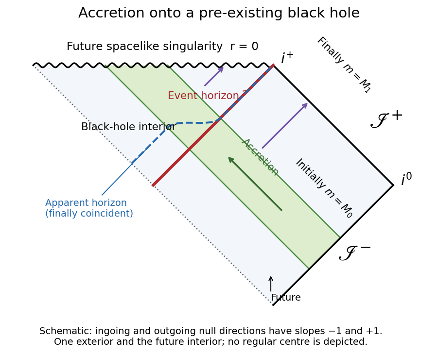
Let $\Delta M=M_1-M_0$ and retain only terms first order in $\mu /M_0$ and $\rho /M_0$. The outgoing event horizon equation expands toHere ${\kappa }_0$ is the initial Schwarzschild surface gravity. The integrating factor $e^{-{\kappa }_{0}v}$ gives $d(e^{-{\kappa }_{0}v}\rho )/dv=-e^{-{\kappa }_{0}v}\mu /(2M_0)$. Future stationarity imposes $\rho =2\Delta M$ for $v>v_0$ and removes the growing homogeneous solution. Integrating from $v$ to infinity yields the teleological response of a Vaidya event horizon:The integral is finite because $\mu$ is bounded. Integrating by parts also givesFor $v>v_0$, this reduces to $2\Delta M$. For $v<0$, the first form becomesConsequently $r_H\to 2M_0$ as $v\to -\infty$. The positive constant $C$ shows that this event horizon is already expanding in the initially vacuum region. For monotone accretion, $\rho -2\mu \ge 0$, so it lies outside the instantaneous apparent horizon to first order. All displayed radius corrections are understood up to $O((\Delta M{)}^2/M_0)$.

The stress-energy tensor is already first order, so its energy flux can be evaluated on the unperturbed Schwarzschild event horizon $r=2M_0$, with the infinity-normalized Killing vector field $\xi ={\partial }_v$. On this background $g^{rv}=1$, and henceThe conserved stress-energy current from a Killing vector is $J^a=-T^a{}_b{\xi }^b$. Its radial component is negative, so the positive inward energy flux is $-J^r$. Using the directed null-surface measure $r_H^{2}dvd\Omega$ givesThe initial and final event horizon areas are $A_0=16\pi M_0^2$ and $A_1=16\pi (M_0+\Delta M{)}^2$. Thus $\Delta A=32\pi M_0\Delta M+O((\Delta M{)}^2)$. With Schwarzschild surface gravity ${\kappa }_0=1/(4M_0)$, the Physical-process first law of black-hole mechanics follows:The flux is Killing energy, including gravitational redshift, rather than the energy measured by a sequence of static observers arbitrarily close to the event horizon.

Locally write the null hypersurface as $S=0$ with $dS\ne 0$, and extend its normal as $n_a={\nabla }_{a}S$. On the hypersurface, $n^a{n}_a=0$, so $n^a{\nabla }_{a}S=n^2=0$: the raised normal is itself tangent. The Levi-Civita connection and symmetry of the scalar Hessian giveAlthough $n^2$ vanishes on the hypersurface, it need not vanish off it. Its tangential derivatives vanish, so ${\nabla }_a(n^2)$ must be proportional to the normal $n_a$. Hence ${\nabla }_{n}n=\kappa n$ on the hypersurface for some smooth local coefficient $\kappa$. The normal's integral curves of a vector field remain in the hypersurface and satisfy the nonaffine geodesic equation. Rescale to $k=hn$, where $n(\log h)=-\kappa$ along each generator. Direct substitution gives ${\nabla }_{k}k=0$. Thus the normal generates null geodesics within the hypersurface, with an affine parameter after this rescaling. This proves the null hypersurface normal generates null geodesics property without incorrectly setting a transverse derivative of $n^2$ to zero.

Choose the affine tangent $k^a$ to a null geodesic congruence, and an auxiliary null vector ${\ell }^a$ with $k\cdot \ell =-1$. The screen-space projectorannihilates $k$ and $\ell$ and restricts to a positive-definite two-dimensional metric in four spacetime dimensions. Neighboring transverse rays have relative displacement governed by the optical tensorIts irreducible decomposition defines the three requested optical quantities:The null expansion $\theta$ is the fractional rate of change of transverse area, $d\log A/d\lambda$. The null shear $\sigma$ changes a beam's shape at fixed area to first order; it is symmetric and trace-free. The null twist $\omega$ is antisymmetric and measures local rotation of the transverse rays; it vanishes for a hypersurface-orthogonal null geodesic congruence. In $D$ dimensions replace $1/2$ by $1/(D-2)$. These definitions use the trace convention for null expansion, rather than the alternative screen-averaged convention.

Take an affinely parametrized null geodesic congruence, ${\nabla }_{k}k=0$. Choose the auxiliary null vector and a transverse orthonormal screen basis to undergo parallel transport along each ray. For the unprojected tensor $C_{ab}={\nabla }_b{k}_a$, the product rule and the Ricci identity yieldHere the Riemann curvature tensor convention is the one in Question 1; its last-index antisymmetry converts the covector commutator to the displayed curvature term. Because $C_{ab}{k}^a=C_{ab}{k}^b=0$, inserting the screen-space projector in the product term adds only terms killed by these contractions. Parallel propagation makes differentiation commute with the screen projection. Therefore, in screen indices $A,B$,This is the optical matrix evolution equation. Its trace has curvature contraction $q^{ab}{R}_{acbd}{k}^c{k}^d=R_{cd}{k}^c{k}^d$: the additional terms in $q^{ab}-g^{ab}$ vanish by curvature antisymmetry. Write $B=(\theta /2)q+\sigma +\omega$ using the null expansion, null shear, and null twist. Symmetric--antisymmetric cross terms have zero trace, $\sigma$ is trace-free, andThe minus sign in the last trace comes from ${\omega }_{ab}=-{\omega }_{ba}$ and the positive screen metric. Taking the trace therefore derives the Null Raychaudhuri equation:For a nonaffine tangent obeying ${\nabla }_{k}k=\kappa k$, the same product-rule derivation adds $+\kappa \theta$ on the right; the projected derivative of $\kappa$ multiplies $k_a$ and vanishes. In $D$ dimensions the quadratic null expansion term is $-{\theta }^2/(D-2)$.

Away from a bifurcation set, the normal to a Killing horizon is its nonzero Killing vector field $K$. Any affine tangent to the same generators has the form $k=hK$. In the optical tensor, derivatives of $h$ contribute a factor of $K_a$ and disappear under the screen-space projector. Consequentlyby the Killing equation. The trace and trace-free symmetric part are therefore zero: $\theta =0$ and ${\sigma }_{ab}=0$.

For the antisymmetric part, locally the horizon normal is proportional to a gradient. The restriction of its dual one-form to every tangent direction on the horizon is zero. Taking its exterior derivative and evaluating on two screen tangents therefore gives zero as well; equivalently this is the hypersurface-orthogonality consequence of the Frobenius theorem. Since both screen indices are tangential, $B_{[ab]}=0$. Thus the optical scalars on a Killing horizon satisfyNo affine normalization of the Killing vector field itself was assumed. At a regular bifurcation surface, $K$ vanishes but the smooth null generators do not; the conclusions for their optical quantities follow by continuity along each horizon branch.

Work initially in units $G=c=\hslash =k_B=1$ and consider gravitational collapse settling to a nonextremal Schwarzschild black hole. Classically, outgoing rays sufficiently close to the forming event horizon suffer an arbitrarily large redshift. Quantum mechanically, the meaning of positive frequency at past null infinity differs from that at future null infinity; a Bogoliubov transformation between these two mode descriptions can therefore mix creation operators and annihilation operators. Hawking's argument computes that mixing and obtains a thermal occupation, even when the incoming state has no particles.

To see why the frequency mixing is universal, use final Schwarzschild time $t$, the Schwarzschild tortoise coordinate $r_{\ast }$, and retarded time $u=t-r_{\ast }$. Near the final event horizon, $r_{\ast }\sim (2\kappa {)}^{-1}\log (r-2M)$, with Schwarzschild surface gravity $\kappa =1/(4M)$. On a fixed advanced-time section, $u=v-2r_{\ast }$, so $r-2M$ is proportional to $e^{-\kappa u}$. Tracing a ray back through the regular collapsing region maps this small separation smoothly to its separation from the last escaping incoming ray. If $U$ is an affine incoming null coordinate and $U_H$ labels that limiting ray, the Hawking exponential ray map isThe logarithm at a simple horizon root fixes the exponent. Smooth propagation through the earlier collapse changes $A$ and phases but not the leading exponential redshift.

For a massless bosonic test scalar field, an outgoing mode of frequency $\omega >0$ at future null infinity behaves as $e^{-i\omega u}$. Trace it backward in the high-frequency geometric optics approximation. Its relevant incoming dependence is, up to normalization and a phase,Here $\Theta$ is the Heaviside step function. Incoming rays with $U>U_H$ do not escape. This truncated logarithmic phase is not purely positive frequency with respect to $U$. Decomposing it into incoming positive-frequency solutions $e^{-i{\omega }^{\prime }U}$ and negative modes $e^{+i{\omega }^{\prime }U}$ gives the Bogoliubov transformation. With $x=U_H-U$, the two relevant Fourier transform integrals areThe former is the positive-frequency coefficient and the latter is the negative-frequency coefficient; the Klein-Gordon inner product introduces the same frequency normalization into their modulus ratio. By the defining integral of the gamma function and analytic continuation in its Laplace parameter,For a complex number $z$ in the right half-plane, $|z^{-1-ia}|=|z{|}^{-1}{e}^{a\arg z}$. As $ϵ\downarrow 0$, the two arguments tend to $+\pi /2$ and $-\pi /2$. This gives the thermal ratio of Hawking Bogoliubov coefficients:The regulator fixes the branches and is essential to the sign of the thermal exponent.

Expand the outgoing annihilator as $b=\int d{\omega }^{\prime }({\alpha }_{\omega {\omega }^{\prime }}^{\ast }{a}_{{\omega }^{\prime }}-{\beta }_{\omega {\omega }^{\prime }}^{\ast }{a}_{{\omega }^{\prime }}^{†})$, including a complete set of incoming channels. The canonical identities for a bosonic Bogoliubov transformation express $[b,b^{†}]=1$. For normalized outgoing wave packets, they give $\int (|\alpha {|}^2-|\beta {|}^2)d{\omega }^{\prime }=1$. In the incoming Fock vacuum, the outgoing mean of the particle number operator is $N_{\omega }=\int |\beta {|}^{2}d{\omega }^{\prime }$. Combining the two identities with the thermal ratio, in the late-time narrow-frequency packet limit, yieldsWave packets avoid interpreting the divergent normalization of infinitely long continuum modes as a finite particle count. The temperature is the Hawking temperature, and the occupation is the zero-chemical-potential Bose-Einstein distribution. Restoring constants, the Schwarzschild black hole temperature is $T_H=\hslash c^3/(8\pi GM{k}_B)$ for physical mass $M$.

The preceding thermal occupation describes the horizon-originating channel before exterior scattering. The exterior angular and curvature potential partly reflects it. For a scalar field, the number flux at future null infinity is consequentlywhere the greybody factor ${\Gamma }_{\ell }$ is the transmission probability of a partial wave. Multiplication by $\omega$ gives its energy flux. Thus the asymptotic spectrum has the thermal denominator but is not an exact blackbody spectrum. For fermionic fields the canonical anticommutation relations replace the minus sign in the occupation denominator by a plus sign, at the same Hawking temperature.

The relevant state is the collapse vacuum for Hawking radiation: no incoming thermal bath at past null infinity, and regular short-distance behavior in freely falling coordinates at the forming event horizon. It predicts an outgoing flux, unlike equilibrium with a thermal bath on an eternal black hole. The derivation uses quantum field theory in curved spacetime on a prescribed classical geometry; it does not require outgoing particles to follow forbidden classical paths out of the interior. Positive energy carried to infinity is accompanied, in the semiclassical description, by negative Killing-energy flux into the black hole. Including that flux in slow backreaction decreases its mass, giving black-hole evaporation.

The approximation applies to the late radiation of a large nonextremal black hole while its surface gravity changes slowly on a time scale ${\kappa }^{-1}$. Backward propagation involves very high locally measured frequencies, so the calculation assumes the usual regular short-distance quantum-field state. It determines the leading radiation and temperature, not the Planck-scale endpoint of black-hole evaporation. The exponential horizon redshift forces positive/negative frequency mixing with a thermal ratio, giving outgoing Hawking radiation at $T_H=\kappa /(2\pi )$.