Cyclic periodicity on implies that the least positive period divides : the shifts preserving the function form a subgroup of the cyclic group. Injectivity within one period says that distinct residue classes modulo have distinct function values. Write .
Prepare the uniform superposition state by applying the quantum Fourier transform to , and evaluate reversibly into a second quantum register. This is efficient because the given classical Boolean circuit can be converted into a reversible circuit, with its workspace cleaned by uncomputation. The resulting quantum state isMeasuring the function quantum register leaves a uniform coset state for some . The amplitude at after a quantum Fourier transform isThe finite geometric series is zero unless is a multiple of , and then equals . Thus a computational-basis measurement produces a uniform Fourier sampleThe exact period recovery from a Fourier sample computesA greatest common divisor is computable in time polynomial in . The candidate is always a divisor of the true period, and equals it precisely when is coprime to .
For the success flag, compute and compare with . If , injectivity within the first period makes these unequal. If , periodicity makes them equal, including . Hence accept and output exactly when this comparison succeeds; otherwise report failure. This is heralded exact quantum period finding when the period divides the register size, with no false acceptance. The case succeeds even on the sample .
The exact success probability iswhere is the Euler totient function. For , the prime-product formula gives . A Rosser–Schoenfeld totient bound supplies the needed lower bound for large . Every single attempt, including verification, has the assumed polynomial-in- gate cost. Repeating times gives constant success probability with a certified result whenever one is found.
The printed in the totient hint should be a lower-bound statement, . Literally, is false: at primes , . Likewise the exact single-sample success probability need not be ; for prime period it tends to one. The useful intended guarantee is the displayed inverse-log-log lower bound, not a universal upper bound. If an algorithm satisfying the literal success upper bound is desired, one can additionally accept an otherwise certified run only when independent fair bits are all zero. This retains a detectable failure flag and polynomial runtime, and has success at most , but deliberately weakens the useful guarantee. The standard unsuppressed algorithm above gives the stronger intended performance. Small can be handled directly. Primary evidence for the totient lower bound is Theorem 15, equations (3.41)–(3.42), in denisevellachemla.eu/Rosser-Schoenfeld-1962.pdf .
Let . The positive-exponent quantum Fourier transform gives . Reindexing the cyclic shift operator givesThus is an eigenstate with eigenvalue , with this sign fixed by the printed quantum Fourier transform convention.
Prepare the first two qutrits in and the answer qutrit in . The modular-addition quantum oracle applies to the answer. Its eigenvalue produces quantum phase kickback, leavingApply to each input qutrit, then measure them in the computational basis. The result isThe preparation, inverse transforms and measurements are independent of , and there is exactly one use of . This is qutrit linear-function identification, the ternary version of Bernstein-Vazirani phase kickback.
Use the bit-query Boolean quantum oracle , where denotes workspace. Initially every probability amplitude is independent of , hence is a constant polynomial. An input-independent unitary gate only forms linear combinations of probability amplitudes, so it does not increase their polynomial degree.
If is an amplitude before a query, its new value isOne query increases polynomial degree by at most one. Inductively, after queries each amplitude has polynomial degree at most . The acceptance probability is a sum of squared absolute values of the accepting amplitudes, so it is a real polynomial of degree at most . Intermediate quantum measurements and classical adaptation can be retained coherently, or handled by summing unnormalized branch probabilities; either approach yields the same degree bound.
An exact algorithm has acceptance probability precisely at every Boolean input. The multilinear reduction on the Boolean cube replaces positive powers of each by , preserving these values without increasing polynomial degree. Therefore the polynomial method for quantum query lower bounds givesHere is the degree of the unique multilinear polynomial representing the Boolean function, and is its exact quantum query complexity. Uniqueness follows, for example, by evaluating successively on the indicator vectors of subsets: the value on a subset determines its coefficient once all smaller-subset coefficients are known.
For the three-bit majority function, the pair products count how many pairs of input bits are both one. Their sum is zero at Hamming weights zero and one, one at weight two, and three at weight three. Subtracting twice the triple product corrects the last value. HenceThis is a multilinear polynomial of degree three, and its top coefficient is nonzero. Uniqueness of the Boolean multilinear polynomial excludes a degree-two alternative. The polynomial method for quantum query lower bounds therefore yields , and the integer number of queries gives
First use the allowed one-query algorithm to learn exactly. This restricted two-index Boolean quantum oracle is realized by relabelling indices in a single query to the original input. Measure its output and choose the second query classically.
If , the first two bits agree and their common value is the majority, irrespective of . Query and output it. If , the first two bits cancel in the vote, so query and output it. ThusThe exact two-query majority algorithm uses one parity query and one ordinary bit query on every branch, and is correct on all eight inputs. Together with the lower bound this proves .
Boolean conjunction is multiplication on zero-one inputs. The block conjunction of three-bit majorities therefore has the multilinear polynomialThe factors use disjoint variables, so their product remains a multilinear polynomial. Its monomial containing all variables has coefficient ; no term has higher degree. By uniqueness, the representing multilinear polynomial has degree exactly . Applying the polynomial method for quantum query lower bounds givesThis argument concerns exact quantum query complexity; the analogous claim for bounded error does not follow from exact polynomial degree.
For a Boolean function , its block sensitivity at is the maximum number of pairwise disjoint nonempty index sets such that flipping all bits in each individually changes . Maximize over to obtain .
Choose , so every three-bit block has majority one and the conjunction is one. In each block, flipping either of its two one bits alone changes that block's majority to zero and therefore changes the conjunction to zero. These singleton index sets are all disjoint, soThe supplied bounded-error quantum query complexity lower bound now givesHere denotes a fixed two-sided error bound below , such as .
In fact the block sensitivity is exactly . At a one-input, selecting two one bits from each triple gives a size- certificate: any block flip changing the output must touch it, so disjoint sensitive sets number at most . At a zero-input, one failing triple contains at least two zero bits; fixing those two zeros certifies zero, so at most two disjoint sensitive sets can change the output. The lower-bound witness above attains . The certificate complexity of a Boolean function supplies these upper bounds, though only the witness is needed for the requested result.
Use five resource qubits, all initially , and prepare the graph state with edges , , , . The labels here identify resource vertices; logical wire 1 travels from vertex 1 to 3, and logical wire 2 travels from 2 to 4 to 5. Each edge is a Controlled-Z gate, and these entangling gates commute, so all can be applied when preparing the resource.
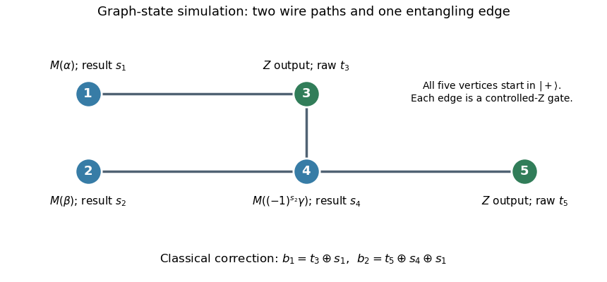
Five-vertex graph resource, adaptive measurement angle, and classical output corrections for the two-qubit circuit
. Details. 
Measure vertex 1 in the equatorial qubit measurement basis at angle , with outcome , and vertex 2 at angle , with outcome . These measurements can be simultaneous. The one-bit teleportation lemma leaves the state on vertices 3 and 4, before the last teleportation, equal up to global phase toIndeed commuting the two initial byproducts through creates precisely the crossed factors. The unused edge from 4 to the fresh vertex 5 is the last one-bit teleportation link.
Measure vertex 4 at angle , with outcome . By the printed J gate propagation identities,Thus the remaining two-qubit quantum state isup to global phase, where is the desired circuit output relabelled onto vertices 3 and 5. The sign choice cancels the unwanted angle reversal caused by the frame on vertex 4.
Finally measure vertices 3 and 5 in the computational basis, obtaining raw results . The Pauli Z gate affects only phases, while the Pauli X gate flips a computational result. The five-vertex graph-state circuit simulation therefore outputsThis deterministic classical correction reproduces the ideal joint probability distribution for every preceding measurement branch. The final fixed-basis measurements may share the second layer with the adaptive measurement of vertex 4, because their projectors act on different vertices; measuring them afterwards is also valid.
Replace every CNOT gate by . The resulting quantum circuit contains only Hadamard gates and Controlled-Z gates. Realize each Hadamard gate by a fresh one-bit teleportation link measured at angle zero, so every internal measurement is in the fixed basis. Insert a graph edge between the current wire vertices for each Controlled-Z gate. This gives a suitable graph state because the inputs are , and entangling gates can be moved to resource preparation: they commute with one another and with earlier measurements on vertices no longer used by the gate.
Track a Pauli frame . An angle-zero one-bit teleportation with raw result updates the frame on that wire bybecause equals up to global phase. A Controlled-Z gate updates and , leaving the bits unchanged. These are classical binary updates; no measurement angle depends on them.
All the internal quantum measurements consequently have predetermined bases. Their projectors act on distinct resource vertices and commute, so all internal measurements can be performed simultaneously: the logical measurement depth is at most one. If the output is to be read in the computational basis, those fixed-basis measurements can occur in the same layer; a raw output is relabelled . If quantum outputs are retained, the same calculation gives the desired output in a known Pauli frame. This nonadaptive Hadamard–CNOT measurement pattern concerns measurement depth, not the depth of resource preparation or classical frame computation.
Write the single-qubit gate as , where . Thus it is, up to global phase, a rotation about the x-axis, and it commutes with . Compile it as a Hadamard gate followed by the J gate . Compile each CNOT gate as before into . The usual wire-link construction yields a resource graph state for the fixed inputs; the same frame algebra also works for logical input states supplied to an open resource.
The point is stronger than counting two gates per rotation: a long circuit must not acquire a new adaptive layer for every rotation. We show that every nonzero-angle basis depends only on outcomes of the angle-zero measurements.
For an gadget, let the incoming Pauli frame be . Denote the angle-zero outcome by , and the subsequent angle- outcome by . The two one-bit teleportations givewhere omits a global phase. Consequently the rotation gadget updatesOnly its angle-zero outcome enters the new frame. Its arbitrary-angle outcome enters only the frame, which commutes through all later gates.
For a CNOT gate from to , call the outcomes of its two angle-zero target-wire measurements , in that order. The Pauli frame update isThese follow by applying the preceding Hadamard gate and Controlled-Z gate frame updates twice. In particular, the new frames depend on old frames and angle-zero outcomes only; they never depend on old frames or arbitrary-angle outcomes. This is the measurement-level version of the given fact that a CNOT gate propagates operators into products of operators.
Starting with no frame, induction in the original circuit order now computes every solely from angle-zero results. Therefore every sign is known after one simultaneous layer containing all angle-zero measurements, including those appearing late in the circuit. Compute those signs classically, and perform all remaining equatorial measurements in a second simultaneous layer. An angle zero that occurs accidentally among these remaining choices may stay in that layer. Reordering is valid because, once a branch's bases have been fixed, the projectors on different vertices commute; no second-layer result is needed to choose another second-layer basis.
The two-layer measurement pattern for CNOT and x-axis rotations thus hasindependently of the number or order of gates. Fixed computational-basis measurements of classical outputs can be included in layer two, followed by relabelling . For quantum outputs the final Pauli frame gives the required correction. The depth statement excludes graph preparation and classical processing, as in the definition in the paper.
Put and prepare control qubits in and the target in the supplied eigenstate . Apply a Hadamard gate to every control qubit. Let denote the integer encoded in that quantum register.
For every , apply a controlled unitary gate with control and the same target. The quantum phase kickback yieldsApplying to the controls therefore produces exactly. A computational-basis measurement returns with certainty, and the algorithm outputsThis is exact quantum phase estimation; exactness uses the finite dyadic phase promise, not a rounding argument.
Only a controlled-U gate is supplied as a primitive. Its repetitions implement controlled-, so the total number of black-box uses is . Access to powers as unit-cost primitives would be a different quantum query complexity model. This distinction is the cost of exact phase estimation on a dyadic spectrum.
The quantum circuit has one control wire per binary digit and one target quantum register. Every control starts in , receives a Hadamard gate, controls the corresponding power , and then enters the collective inverse quantum Fourier transform. Only the control register is measured; the target stays in .
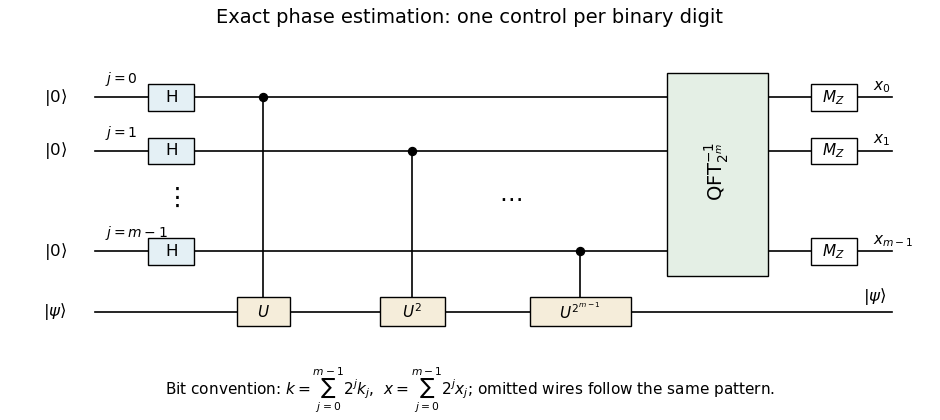
Exact dyadic phase-estimation circuit with controlled powers, inverse Fourier transform, and little-endian output bits
. Details. 
The omitted intermediate wires continue the pattern . The inverse quantum Fourier transform black box is defined on the integer basis with , so the displayed ordering introduces no hidden bit reversal. The measured bits satisfyEach controlled power box represents sequential controlled- uses when only that primitive is available.
Let . In terms of the Pauli X gate, the given unitary operator is , with and . Since and ,Thus the normalized eigenvectors are , with eigenvalues and respectively. At they coincide as eigenvalues, and the whole two-dimensional Hilbert space is the eigenspace; the same chosen eigenbasis remains valid.
Prepare independently of and use the exact quantum phase estimation circuit of the preceding parts on the controlled- black box. It returns exactly usingThe chosen eigenstate contains all the unknown phase information, unlike , whose eigenvalue is independent of .
Again put , . If computational strings differ in places, the matrix element of between them is : an unchanged bit contributes , and a flipped bit contributes . Hence the given operator isThe printed factored expression is undefined at , namely . Its polynomial form gives the natural continuous extension there, . For the strict promise avoids that singular value; for the extension is needed to include the allowed phase . This is a removable defect of the formula, not a failure of unitarity of the tensor-product operator.
Prepare . Its eigenvalue is , giving tensor-product eigenphase amplification. Write . If , thenwhere the upper bound is exactly the promise . Thus the amplified phase has only unknown binary digits and no modulo-one aliasing. Run exact quantum phase estimation with controls on the controlled- black box. It returns exactly, after which division by the original recovers .
The number of joint black-box uses isIf , the dyadic promise and force , so output without querying the oracle. This covers the zero-control edge case without an invalid negative number of phase bits. The improvement counts one supplied controlled- call as one query. Implementing such a joint call from individual controlled- calls would remove the claimed factor- primitive-query saving, and preparing the target qubits is a separate gate cost.
Articles by others on the same topic
There are currently no matching articles.