Past exam of the mathematics course of the University of Cambridge / 2013 / iii / Paper 64 (Image Processing --- Variational and PDE Methods)

Write $\mathrm{TV}(u)=|Du|(\Omega )$ for the total variation seminorm on a domain. For a locally integrable real function its dual definition isThe bounded-variation space consists of functions $u\in L^1(\Omega )$ with finite $|Du|(\Omega )$, equipped with $\Vert u{\Vert }_{BV}=\Vert u{\Vert }_1+|Du|(\Omega )$. In the equivalent distributional derivative description, $Du$ is a finite vector-valued Radon measure and $|Du|$ is its total variation measure.

To establish completeness of the bounded-variation space, let $(u_n)$ be Cauchy in this norm. Completeness of $L^1$ gives $u_n\to u$ in $L^1$. Given $\epsilon >0$, choose $N$ so that $\Vert u_n-u_m{\Vert }_{BV}<\epsilon$ whenever $m,n\ge N$. For fixed $n\ge N$, the given lower semicontinuity yieldsSince $\Vert u_n-u_m{\Vert }_1\to \Vert u_n-u{\Vert }_1$, we obtain $\Vert u_n-u{\Vert }_1+|D(u_n-u)|(\Omega )\le \epsilon$. In particular $u_n-u$ has finite variation; the triangle inequality then puts $u$ in the BV space. The same bound proves convergence in the full norm, so this is a Banach space.

For the disk data, put $B=B(0,R)$ and assume $\alpha >0$. The exact total variation denoising of a disk isHere $(s{)}_{+}=\max (s,0)$ is the positive part. A total variation calibration certifies global optimality, including competitors that are not radial or piecewise constant. Define the bounded vector fieldIt has $|z|\le 1$. Its normal component is continuous across the circle, so the distributional divergence has no extra boundary measure. Direct differentiation gives $q=\mathrm{div}z=(2/R){\chi }_B$. The dual definition implies $\int vq\le \mathrm{TV}(v)$: for the standard $BV\cap L^2$ domain one can cut $z$ off at radius $L$, with the error bounded by $C{L}^{-1}{\int }_{L<|x|<2L}|v|\to 0$, and then smooth the test field. In the larger homogeneous bounded-variation space, the same error is bounded by $C\Vert v{\Vert }_{L^2(L<|x|<2L)}\to 0$. Thus both usual whole-plane formulations give the same certificate.

Use the perimeter identity $\mathrm{TV}({\chi }_B)=2\pi R$ and $|B|=\pi R^2$. If $c=1-2\alpha /R>0$, then $\int c{\chi }_{B}q=2\pi Rc=\mathrm{TV}(c{\chi }_B)$ and $u_{\ast }-g+\alpha q=0$. Consequently every competitor $v$ satisfiesIf $\alpha \ge R/2$, replace $z$ by $z_{\alpha }=(R/(2\alpha ))z$. Its norm is still at most one, its divergence is $q_{\alpha }={\chi }_B/\alpha$, and equality in the calibration holds at $u_{\ast }=0$. The identical comparison proves optimality and uniqueness of zero, including the threshold $\alpha =R/2$. The only general results used are completeness of $L^1$, lower semicontinuity of variation, the indicator-perimeter identity, the distributional integration-by-parts/dual variation formula and the quadratic norm identity. For $\alpha =0$, the unique squared-error minimizer is simply $g$.

Positivity means $u>0$ almost everywhere, since the real logarithm must belong to $L^1$. A positivity-preserving operator gives $s=Tu\ge 0$. For fixed $x$, the scalar shifted Poisson data fidelity is $f_x(s)=s-g(x)\log (1+s)$, withComposition with the linear operator $T$ proves convexity in $u$, and strict convexity holds along pairs whose forward images differ on a set of positive measure. The admissible class itself is convex: the concavity of the logarithm gives $\log (\theta u+(1-\theta )v)\ge \theta \log u+(1-\theta )\log v$, controlling its negative part, while ${\log }^{+}w\le w$ controls its positive part.

Because $|\Omega |=1$ and $\log (1+s)\ge 0$, the Jensen inequality gives the requested bound:The final equality uses nonnegativity and the unit area. Since $t-G\log (1+t)\to \infty$, this controls the forward-image norm on energy sublevels.

The printed strictly positive problem has no minimizer. This is nonattainment under strict positivity for shifted Poisson fidelity, rather than a failure of the coercivity calculation. Indeed, with $0<g<1$ and $s>0$, $\log (1+s)<s$ implies $f_x(s)>0$. Also $Tu$ cannot vanish identically for a strictly positive $u$. To see this, let $E_n=\{u\ge 1/n\}$. If $Tu=0$, positivity and $0\le {\chi }_{E_n}\le nu$ give $T{\chi }_{E_n}=0$. But ${\chi }_{E_n}\to {\chi }_{\Omega }$ in $L^1$ and continuity of $T$ would imply $T{\chi }_{\Omega }=0$, contradicting the hypothesis. Thus every admissible $u$ has positive fidelity and hence positive total energy.

Conversely, the constants $u_{\epsilon }=\epsilon {\chi }_{\Omega }$ are admissible, have zero total variation, and satisfyTheir logarithms are integrable for each $\epsilon >0$, but the limit is excluded. ThereforeA bounded minimizing sequence and bounded-variation compactness do not repair a nonclosed positivity/logarithm constraint. In particular, a literal existence or uniqueness proof for that domain is impossible.

The natural correction is to minimize over $BV(\Omega )$ with $u\ge 0$, omitting the unnecessary $\log u\in L^1$ condition: the fidelity only contains $\log (1+Tu)$, which is already integrable. Here is the full existence for nonnegative shifted Poisson regularization argument, also valid for any bounded nonnegative data $g$. Let $G=\Vert g{\Vert }_{\infty }$, $m_G={\inf }_{t\ge 0}\{t-G\log (1+t)\}>-\infty$, and take a minimizing sequence of energy at most $C$. The displayed bound gives $\Vert T{u}_n{\Vert }_1\le C_1$ and $\alpha \mathrm{TV}(u_n)\le C-m_G$. Write $c_n={\int }_{\Omega }{u}_n\ge 0$. The Poincaré inequality for total variation and mean control for positive imaging operators yieldThe denominator is nonzero, so the full $BV$ norm is bounded. Bounded-variation compactness gives $u_n\to u$ in $L^1$ along a subsequence, with $u\ge 0$. Continuity gives $T{u}_n\to Tu$ in $L^1$. On $s\ge 0$, $|f_x^{\prime }(s)|\le 1+G$, so the fidelity converges in the integral; lower semicontinuity of variation completes the direct method in the calculus of variations.

For the actual printed data $0<g<1$, the corrected problem has the unique minimizer $u=0$, even if $T$ is not injective. Zero attains energy zero. Any other zero-energy candidate would have both $Tu=0$ and $\mathrm{TV}(u)=0$; on the connected square, zero variation makes $u$ a nonnegative constant, and $T{\chi }_{\Omega }\ne 0$ forces that constant to vanish. For general positive bounded data, an injective $T$ is a sufficient uniqueness condition, because its fidelity is strictly convex; injectivity is not a necessary condition in every instance.

In the finite-dimensional interpretation, let ${\lambda }_{ij}=1+(Tu{)}_{ij}$. Independent Poisson observations with these intensities have negative log-likelihood ${\sum }_{ij}[{\lambda }_{ij}-g_{ij}\log {\lambda }_{ij}]+C(g)$. Removing the constant $\sum 1$ gives precisely the stated fidelity. Thus the model is Poisson counting noise with a unit background intensity, or an approximate version of it for rescaled/continuous grey values. Literal Poisson counts are integers; the constraint $0<g<1$ is a grey-value normalization, not a literal unscaled count sample.

The bounded classical solution is the heat-kernel convolutionThe two-dimensional heat kernel has integral one. Boundedness of $g$ permits differentiation under the integral for $t>0$, proving $u_t=\Delta u$ and $|u|\le \Vert g{\Vert }_{\infty }$. Its approximate identity property gives $u(x,t)\to g(x)$, locally uniformly since $g$ is continuous. This bounded solution satisfies the required Gaussian-growth bound.

For heat-equation uniqueness under Gaussian growth, let $w$ be the difference of two solutions, so $w(x,0)=0$ and $|w|\le M_0{e}^{a|x{|}^2}$ on a finite time interval. Choose $b>a$ and a slab $0\le t\le \tau <1/(4b)$. The positive comparison solutionsatisfies $({\Phi }_b{)}_t=\Delta {\Phi }_b$. For any $\epsilon >0$, its faster spatial growth makes $|w|\le \epsilon {\Phi }_b$ on a sufficiently large lateral cylinder boundary. At the initial boundary, $w=0$. The heat equation maximum principle applied to $\pm w-\epsilon {\Phi }_b$ proves the same inequality inside. First allow the cylinder radius to increase, then let $\epsilon \downarrow 0$. Repeating these slabs proves uniqueness on every finite interval with the stated uniform growth bound. No spatial integrability of $g$ is required.

At time $T$, this is Gaussian filtering with covariance $2TI$, hence $\sigma =\sqrt{2T}$ per coordinate. With the angular-frequency Fourier transform convention $\hat{f}(\xi )=\int e^{-ix\cdot \xi }f(x)dx$, the Gaussian filtering Fourier multiplier isFor merely bounded $g$, this identity is understood through tempered distributions. The multiplier leaves the zero frequency unchanged and attenuates large frequencies exponentially: it suppresses rapid noise fluctuations but blurs image edges. In cycles-per-length frequency $k$, the multiplier is $e^{-4{\pi }^{2}T|k{|}^2}$.

For the printed Perona-Malik equation, retain the supplied conductance $c(s)=s{e}^{-s^2/(2{\lambda }^2)}$, which includes an extra factor $s$. In one dimension write $p=u_x$ and $F(p)=c(|p|)p=p|p|e^{-p^2/(2{\lambda }^2)}$. Then $u_t=F^{\prime }(u_x)u_{xx}$, withThe forward-backward threshold for gradient-weighted exponential diffusion is thereforeAt $|u_x|=0$ and $\sqrt{2}\lambda$ the coefficient vanishes, giving degenerate diffusion. Increasing $\lambda$ increases the forward-diffusion range. Small nonzero slopes smooth, while large slopes formally sharpen; a negative coefficient produces short-wave growth and ill-posedness, so this is a dynamics explanation, not a general existence theorem for arbitrary data. Replacing the printed conductance by $e^{-s^2/(2{\lambda }^2)}$ would give threshold $\lambda$, but that is a different equation.

The four-neighbour mean expansion follows by Taylor expansion: opposing first and third derivatives cancel, soIf $u(x_0)={\mathrm{mean}}_h(u)(x_0)$ for every sufficiently small $h$, division by $h^2$ and passage to the limit give $\Delta u(x_0)=0$. This is a pointwise conclusion; it does not assert harmonicity in a whole neighbourhood.

For the area median over the disk, the disk-median curvature expansion, at a point where $|\nabla u|\ne 0$, isConsequently the analogous median fixed-point condition yieldsThis is the vanishing of the level-line curvature at $x_0$: to second order the level line is straight there. It need not be a straight segment. For example $u(x,y)=y+x^3$ has zero disk median at the origin for every radius, by odd symmetry, but its zero level line is the cubic $y=-x^3$. Vanishing curvature on an entire connected regular level arc would force that arc to be straight. The factor $1/6$ is for the disk's uniform area measure; a circle-boundary median has a different scale factor, while producing the same zero-curvature equation.

An image segmentation separates an observed image signal into regions that are smooth within themselves and separated by meaningful image edges. Pure image smoothing blurs the very transitions that ought to define these regions. The Mumford–Shah segmentation model instead chooses the reconstruction and its discontinuity set together. For a bounded planar Lipschitz domain and bounded grey-value data $g$, one standard normalization isHere $K$ is the relatively closed edge set and $u\in H^1(\Omega \setminus K)$ can have different traces on its two sides. The first term is quadratic fidelity, the second penalizes variation within regions, and the Hausdorff measure term charges total edge length. It balances fitting, denoising and economical region geometry. The model was developed by David Mumford and Jayant Shah; their 1989 paper formulates this joint variational approach.

All three terms matter. Without fidelity, a constant reconstruction with no edge has zero energy. Without the gradient term, smooth data can be fitted exactly with no edge penalty. Without the length term, fine partitions with nearly constant region means can drive fidelity arbitrarily low while creating excessive boundaries. This is segmentation overfitting without an edge penalty. Increasing $\alpha$ favors flatter regions; increasing $\beta$ makes extra boundaries more expensive and can remove small features. These parameter effects describe a balance, not a guaranteed monotone evolution of every individual boundary.

For fixed $K$, varying $u$ gives the fixed-edge Euler-Lagrange equation for Mumford–Shah:The boundary condition is a separate one-sided Neumann boundary condition on each side of an edge, not continuity of $u$ across it. The fidelity makes this fixed-edge problem strictly convex, so its weak solution is unique by the Lax-Milgram theorem. Optimizing the edge set remains a different geometric problem. The nonconvexity of Mumford–Shah segmentation prevents a general uniqueness assertion or a guarantee that a numerical stationary point is globally optimal.

The piecewise-constant Mumford–Shah problem imposes $u=c_i$ on regions $E_i$. It minimizesThe factor $1/2$ counts each shared internal boundary once. The region means in piecewise-constant segmentation give $c_i=|E_i{|}^{-1}{\int }_{E_i}g$, provided $|E_i|>0$. Thus the remaining optimization concerns the partition. For a smooth interface between $i$ and $j$, moving it in the normal pointing out of $i$ changes fidelity by $[(c_i-g{)}^2-(c_j-g{)}^2]$ per unit displacement, while length changes by its curvature $\kappa$. The resulting segmentation interface curvature balance isWith equal isotropic interface costs, three freely meeting smooth edges satisfy the triple-junction angle in isotropic segmentation: force balance of their unit tangents gives angles of $120$ degrees. These are local stationarity conditions on regular interfaces, not a description of every singular edge configuration.

A simple piecewise-constant segmentation contrast threshold explains why small objects can disappear. On a domain of area $A$, suppose two constant intensities differ by $d$, occupying areas $a$ and $A-a$ with internal boundary length $L$. Keeping that boundary fits the data exactly and costs $\beta L$. Merging both regions costs the within-region squared error $a(A-a)d^2/A$. Among these two candidates, splitting wins precisely when $\beta L<a(A-a)d^2/A$. Other partitions may beat either candidate, so this is not a universal global segmentation formula.

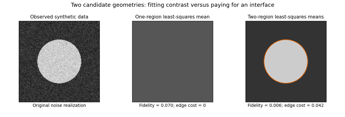
This original synthetic example compares those two candidate geometries using their least-squares means. It illustrates the edge cost; it does not claim to compute the globally optimal Mumford–Shah segmentation.

Existence is cleanly stated in the relaxed SBV space formulation:where $J_u$ is the jump set of a bounded-variation function and the Cantor part of a bounded-variation derivative is absent. Clip a minimizing sequence to the bounded data range: this cannot increase fidelity, gradient energy or jump length. Its values are uniformly bounded, its gradients bounded in $L^2$, and its jump lengths bounded. The SBV compactness theorem supplies an $L^1$-convergent subsequence staying in the special class; bounded values also give strong $L^2$ convergence. The fidelity then converges, while gradient energy and jump length are lower semicontinuous. The direct method in the calculus of variations produces a minimizer. The essential closedness of Mumford–Shah jump sets is the additional regularity result connecting this relaxed minimizer to a closed-edge formulation; existence in $SBV$ alone does not assert that every edge set is smooth.

A practical continuous approximation is the Ambrosio–Tortorelli approximation, introduced in Ambrosio and Tortorelli's 1990 paper. An auxiliary field $v\in [0,1]$ is near one in regions and near zero at edges. One normalized energy isThe edge field weakens smoothing across a narrow transition, and its own energy approximates interface length. The Gamma-convergence result, together with the required compactness, relates global minimizing sequences to the limiting segmentation energy; it does not make the finite-parameter problem jointly convex. Alternating the two fields solves quadratic elliptic subproblems, but initialization and stopping can affect which local stationary configuration is found. The strengths of the model are joint denoising and segmentation, sharp transitions and a geometric cost. Limitations include competing local minima, sensitivity to scale parameters, loss of fine texture, and boundaries driven by intensity rather than semantic object identity.