Past exam of the MPhil in micro- and nanotechnology enterprise course of the University of Cambridge / 2017 / Paper 1 / Section A(i)

The electron-optical column contains an electron gun, an accelerating supply, a condenser lens system, an objective aperture, an electron objective lens, scan coils and alignment/stigmation controls. The electron gun may use thermionic emission or field emission. The condenser lens system sets the incident probe current and source demagnification; the electron objective lens focuses the probe on the specimen. A movable specimen stage controls position, tilt and working distance. The column and specimen chamber need a vacuum system, appropriate pumps and specimen-transfer hardware. Detectors collect secondary electrons, backscattered electrons or characteristic X-rays; amplification and synchronized raster acquisition assign a measured signal to each image pixel. The first two signals provide different imaging information, while characteristic X-rays allow elemental analysis. A source, probe-forming optics, raster scan, specimen stage, detectors, acquisition electronics and vacuum system form the essential chain.^[ref]

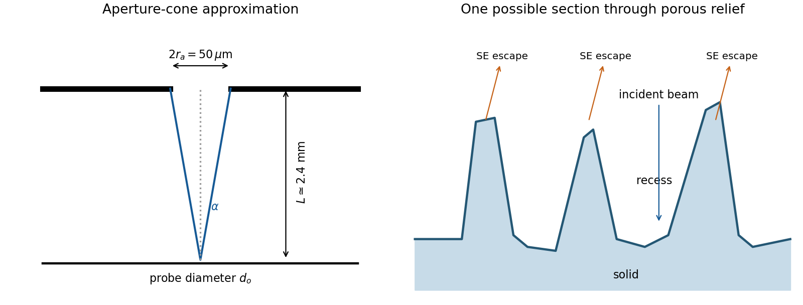
The image annotation gives probe electric current $I=43\mathrm{pA}=4.3\times 10^{-11}\mathrm{A}$ and working distance $L=2.4\mathrm{mm}$. Interpret $d_o$ as the probe diameter and $\alpha$ as its convergence semiangle, in radians. To estimate that angle from the available dimensions, approximate the effective aperture plane as a distance $L$ from the specimen. With aperture radius $r_a=25\mu \mathrm{m}$,The electron beam brightness $\beta$ measures electric current per probe area per solid angle; the supplied convention corresponds to a circular probe and a paraxial cone of solid angle approximately $\pi {\alpha }^2$. The aperture diameter must be halved, and the annotated current is in picoamperes. Treating the full aperture angle as $\alpha$ would introduce a factor-of-two error in $d_o$.

This is a conditional optical estimate: the working distance is not necessarily the actual electron-optical distance from the effective aperture to the focused probe. The answer assumes that approximation, the quoted electron beam brightness at the operating voltage, and negligible optical aberrations. The 30 kV annotation gives a much shorter de Broglie wavelength than 4 nm, so a nanometre-scale probe is plausible. Actual electron microscope resolution also depends on diffraction, scattering in the specimen, signal generation and collection, signal-to-noise ratio, drift and specimen charging. A 4 nm probe does not establish that every measured edge width is 4 nm.

The SE annotation identifies a secondary electron image. The specimen has an open network of ridges, thin walls and irregular cavities, with lateral features on the scale of tens to hundreds of nanometres when compared with the 500 nm bar. Exposed edges can emit secondary electrons from more than one nearby surface; inclined faces also have a larger near-surface escape fraction than a face perpendicular to the beam. These mechanisms make protruding rims conspicuous. Recesses can be dark because emitted secondary electrons are intercepted or collected less efficiently. A through-lens detector changes the collection geometry, so a simple one-sided illumination analogy is incomplete.^[ref]

An irregular porous relief with bright rims and darker recesses is consistent with the image. The cross-section below is an original illustrative geometry, rather than a reconstruction of a particular image line. A single secondary electron intensity map does not supply calibrated heights, prove that every dark patch is a through-hole, or distinguish charging from all material contrast. Repeat with specimen tilt, altered detector collection or reduced accelerating voltage, and compare backscattered electron or elemental signals before assigning a compositional cause.

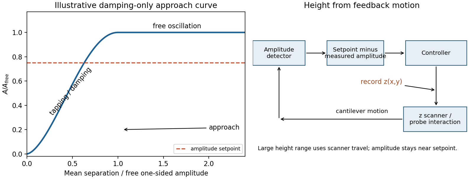
Model the AFM cantilever as a driven damped harmonic oscillator. If the drive stays at the free-space resonance and the spring constant $k$ and effective mass $m$ are unchanged, its steady amplitude isHere ${\gamma }_0$ is intrinsic damping and ${\gamma }_{\mathrm{ts}}$ the added dissipative interaction with the surface. At large average separation there is no tapping, so ${\gamma }_{\mathrm{ts}}\simeq 0$ and $A=A_{\mathrm{free}}$. As the lower turning point reaches the surface, intermittent contacts dissipate energy and the amplitude decreases. With further approach the oscillation becomes strongly constrained, eventually approaching a continuously contacting, nearly quenched response. The damping-only sketch has a free-amplitude plateau followed by a descending amplitude on approach. The rounded transition in the sketch is illustrative; adhesion and actual contact mechanics determine its shape. The deliberately omitted force-gradient-induced resonance shift can make real approach curves more complicated.

An uncorrected amplitude image has a useful vertical range only across the transition between free oscillation and strongly suppressed oscillation. If the free motion is a few tens of nanometres peak-to-peak, its one-sided amplitude is half that excursion. The relevant vertical height range is therefore of the order of the oscillation excursion, only tens of nanometres, rather than micrometres. It is not a sharp universal limit equal to the quoted peak-to-peak value: the chosen mean gap, contact law and usable sensitivity determine the actual range. A sufficiently high feature can quench the motion or produce destructive contact; a sufficiently deep depression leaves the probe oscillating freely with essentially no height sensitivity. This argument limits height tracking, not the lateral width of a feature. Lateral resolution instead depends on AFM tip convolution, sampling and the probe-surface interaction.

In tapping-mode atomic force microscopy, demodulate the cantilever displacement to obtain its amplitude and compare it with a setpoint below $A_{\mathrm{free}}$. A closed-loop control system drives a piezoelectric scanner in $z$ to restore the setpoint as the raster crosses raised or depressed regions. The interaction remains in its sensitive amplitude range while the scanner follows heights much larger than the oscillation amplitude. The principal height image is the calibrated feedback $z$ displacement at each lateral pixel. The amplitude-error and phase channels are supplementary signals, rather than interchangeable height measurements. Maximum height is now bounded by scanner travel, clearance and stable tracking. Steep features require adequate feedback bandwidth and sufficiently slow scanning; trace/retrace disagreement tests tracking, while a changed AFM probe tests geometric broadening. Surface-dependent dissipation can move the setpoint height even on a geometrically flat specimen.