At the current point , a trust-region method approximately minimizes a local quadratic modelwhere is a symmetric Hessian approximation and is the trust-region radius. For a step with positive predicted decrease, compare the true and predicted reductions throughChoose fixed thresholds . If , the step is unsuccessful: reject it and reduce the radius. If , accept the successful step and normally retain the radius. If , the step is very successful: accept it and permit an increase in radius, especially when the step reaches its boundary. The ratio tests whether the local model is accurate enough to justify moving. An approximate subproblem solver should deliver at least the model decrease achieved at the Cauchy point.
The Cauchy point minimizes the model along the negative-gradient ray within the ball. For , write , . Thenwhose scalar minimum occurs at unless the ball cuts the ray short. ThereforeIf , its predicted decrease is . Otherwise it is . Thus every feasible step with satisfies the Cauchy decrease boundFor , take ; the bound reduces to zero.
The global optimality conditions for a quadratic trust-region subproblem with Hessian are: for some ,Here , so the shifted matrix is positive definite. If , choose and . If , the active boundary gives and . HenceThis is exactly the Cauchy point. Because the model is strictly convex, it is the unique global minimizer, including when .
The true quadratic has and the exact expansionSubtracting the model with Hessian yields . Since is symmetric positive definite and , its eigenvalues lie in , so . ThereforeIn fact the stated assumptions give a factor one-half better than the requested bound.
Write for the predicted decrease, assuming a nonstationary point and a step at least as good as the Cauchy point. When , part (ii) gives . Part (iv), using its weaker requested bound, then givesConsequently implies .
For the radius conclusion, use the standard update rules from part (i). Suppose no subsequence of the generated gradient norms tends to zero. Then some bounds those norms below eventually. If , eventually , so every subsequent step is very successful by the preceding estimate. The radius is then maintained or increased, contradicting convergence to zero. Hence a radius tending to zero forces a subsequence of gradient norms to tend to zero. The conclusion uses the trust-region update rules as well as the model estimates.
Use the optimization Lagrangian and let be the constraint Jacobian matrix. Under the standard regularity hypothesis , a local constrained minimizer satisfies, for some multiplier ,The second-order necessary condition isRegularity makes each such tangent vector the velocity of a feasible smooth curve. Twice differentiating the objective along that curve and using stationarity and the differentiated constraints gives the displayed nonnegative second derivative.
The regularity hypothesis is needed for these multiplier conditions to be necessary in this form. For example minimizing subject to has the unique feasible minimizer zero, but for every . The question does not explicitly state the qualification, so it must be supplied when using the usual KKT conditions.
The sequential quadratic programming step minimizes a quadratic local objective model while enforcing the first-order constraint expansion . When the iterate and multipliers are close to a regular solution and approximates the Lagrangian Hessian, the resulting correction approximates a Newton step for the nonlinear KKT conditions.
Full row rank of ensures that is solvable for every and that the multiplier of the quadratic subproblem is unique. A positive-definite makes the objective strictly convex and coercive on the affine feasible set, giving a unique global subproblem minimizer. In fact positivity on , rather than on every vector, is enough for uniqueness and boundedness on that set; full positive definiteness is a convenient stronger assumption.
Stationarity of the equality-constrained quadratic subproblem gives . Together with feasibility, this isMultiplying the bottom block row by gives a symmetric indefinite saddle-point matrix, with right side .
One solution strategy uses the Schur complement. From obtainThis is an positive-definite system when has full row rank; factor and solve with it rather than forming its inverse.
A second strategy uses a nullspace basis for . Choose one particular with , write , and solve the reduced systemThe reduced Hessian is positive definite. These range-space and nullspace reductions exploit different relative sizes of and .
Since is even, differentiating givesAt a stationary point define . Then , precisely the stationarity equation for the optimization Lagrangian. Bounded multipliers giveThus along any subsequence of stationary points with , a further subsequence of bounded multipliers converges to , and continuity yields and . These are the equality-constrained first-order conditions. Bounded multipliers alone do not establish convergence of the primal points; the precise conclusion concerns their finite cluster points. This is the power penalty multiplier limit.
Suppress the iteration subscript. From the quadratic subproblem, and . ThereforeWhen , the stated bound on makes . Consequentlyusing positive definiteness of . Thus every nonzero such SQP step is a descent direction for the penalty function. If , the quotient bound is unnecessary and the same conclusion follows for every . A zero step has zero directional derivative and is not a strict descent direction; it corresponds to an already feasible stationary point. This nonzero-step qualification is implicit in the requested conclusion.
For , the unit steepest descent direction is by the Cauchy-Schwarz inequality. The usual unnormalized direction is ; choosing its scale separately as a line-search step gives the same ray. It satisfies , so it is a descent direction. The first-order Taylor expansion then guarantees decrease for sufficiently small positive steps. The subsequent bounds use this unnormalized negative-gradient convention.
A Lipschitz gradient with constant gives the descent lemmaFor , this upper bound is at most whenever . Since is a descent direction, the right side is positive. Thus the Armijo condition holds throughoutAt it holds by equality. If the gradient Lipschitz constant can be taken as zero, the objective is affine and every positive step along a descent direction passes this sufficient-decrease test.
The backtracking line search starts with , tests the Armijo condition, and repeatedly replaces a failed step by , with fixed . It accepts the first step that passes. Backtracking makes an overambitious trial step small enough for a local linear model to predict the change reliably; part (ii) ensures finite termination. The Armijo condition guarantees a decrease of at least along a nonzero descent direction. Merely obtaining some decrease without this quantitative lower bound would not provide the convergence estimate in the following parts.
For , part (ii) simplifies to . If the initial step is accepted, . Otherwise the immediately preceding trial failed and hence exceeded . ThereforeThe fixed global Lipschitz constant and search parameters make this lower bound uniform across iterations. At , the zero update passes the first trial and the sequence can be kept stationary.
The Armijo condition with gives . Summing these inequalities telescopes toIf , these partial sums of nonnegative terms are bounded above by . The resulting series converges, so its terms tend to zero: .
Use the uniform lower step bound from part (iv):Thus . This is convergence to stationarity in the usual global convergence theorem for the steepest descent method. It does not itself prove that the iterates converge, or that any stationary limit is a global minimizer of a nonconvex objective.
Two reasons to prefer more advanced methods for smooth, high-accuracy optimization are:
- Slow progress on ill-conditioned problems. On an elongated quadratic level set, successive negative gradients can zigzag across the narrow valley. Convergence can be only linear with a factor close to one, and line search cannot remove the underlying poor scaling.
- Failure to retain curvature information. Each new step again uses only the current gradient. Newton's method and quasi-Newton methods exploit curvature to obtain substantially faster local convergence under suitable hypotheses, often compensating for their more expensive steps.
The question's blanket wording is too strong: the steepest descent method and related gradient algorithms are used in practice, especially when problem size, cheap gradients or simplicity make curvature-based alternatives costly. The objections describe limitations, not universal nonuse.
With , the Karush-Kuhn-Tucker conditions areUnder a suitable constraint qualification, such as the linear independence constraint qualification on active constraint gradients, they are necessary for a local minimum. Smoothness alone is insufficient. The sign convention here corresponds to constraints written as and a minus sign in the optimization Lagrangian.
Write the constraint as and its multiplier as . The KKT conditions becomeIf is positive definite, is positive definite for every , so is the only critical point.
For indefinite , the origin remains a critical point, contrary to an unqualified reading of the question. Every nonzero critical point is an eigenvector with , so its eigenvalue is nonpositive. A negative-eigenvalue vector must lie on the unit sphere, with multiplier equal to the negative of that eigenvalue. A nonzero vector in may have any norm at most one and has multiplier zero. Positive-eigenvalue directions do not satisfy the multiplier sign condition. These first-order critical points include saddles; the global minimum selects a unit vector in the lowest-eigenvalue eigenspace.
The logarithmic barrier isIts gradient is . Thus every nonzero stationary point satisfiesA fixed negative-eigenvalue branch exists for . The zero point is stationary for every as well, and it is not an eigenvector; at zero the displayed scalar need not be an eigenvalue of . Thus the claimed eigenvalue conclusion requires the nonzero-point qualification. This distinction is essential for the following Hessian analysis.
Put . Differentiating the barrier gradient givesAt a nonzero stationary point on the branch , . Choose an orthonormal eigenbasis of the symmetric matrix whose first vector is . On each of the remaining eigenvectors the rank-one term vanishes, so the corresponding Hessian eigenvalues areAlong , the first two terms cancel and the remaining eigenvalue isIf repeats, a transverse eigenvalue can be zero. If a lower eigenvalue than exists, a transverse eigenvalue is negative, identifying this stationary branch as a saddle rather than a minimum.
Along a fixed nonzero branch, and the radial Hessian eigenvalue grows like . The nonzero transverse eigenvalues stay fixed. If is simple, the ratio of the largest to smallest absolute eigenvalue therefore tends to infinity. If it repeats, the Hessian is already singular because of the zero transverse directions; there is no finite spectral condition number to begin with. These conclusions concern the nonzero branches: at the stationary origin , and the same blowup is not implied.
Ill-conditioning does not invalidate barrier minimizers as approximations to the constrained solution. Let . At radius , the smallest possible quadratic value is , so global barrier minimization reduces to minimizing for . For its unique minimizing radius satisfiesThus every limiting unit vector in that eigenspace solves the original problem, with objective . For the barrier minimizer is the origin instead. The increasing condition number concerns the numerical difficulty of small-parameter subproblems, which can call for scaling or a primal-dual interior-point method; it does not prevent the mathematical convergence just established. This is the quadratic-ball barrier eigenvalue branch.
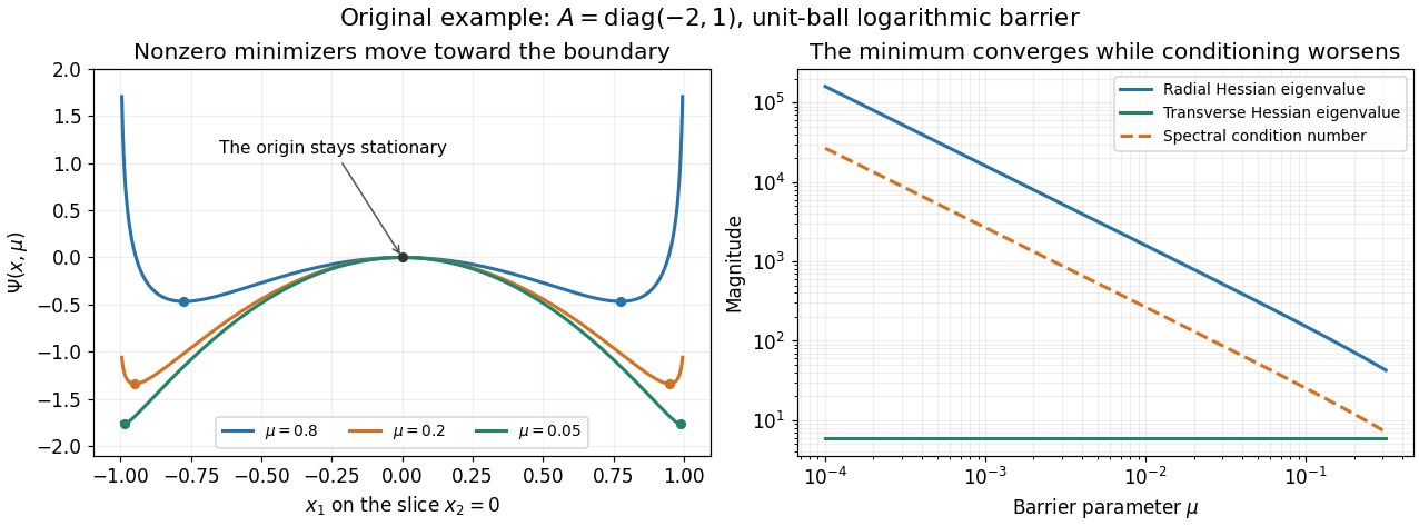
The nonzero barrier minimizers approach the unit sphere while their Hessian condition number grows; the origin remains stationary
. Details. 
Articles by others on the same topic
There are currently no matching articles.