Past exam of the physics A course of the University of Cambridge / 2010 / Paper 2 / Section A

As an estimate, model the confinement by an infinite square well of width $L$ and use the stipulated electron mass. Its energy eigenvalues are $E_j=j^2{\pi }^2{\hslash }^2/(2m{L}^2)$, $j=1,2,\dots$, so the gap controlling thermal occupation of a quantum well isThus $T\ll 130\mathrm{K}$ suppresses excitation: $p_2/p_1=e^{-\Delta E/(k_{B}T)}$. For example $T\lesssim 28\mathrm{K}$ makes this ratio below one percent in this model. There is no sharp cutoff. The ground state energy itself corresponds to about $44\mathrm{K}$, but it is the excitation gap that enters the Boltzmann factor. Finite barrier height and a different effective mass would change the numerical scale; neither is supplied.

For normalized amplitudes $c_n,c_{n^{\prime }}$ and a time-independent observable $A$, the Schrödinger equation givesThe interference term therefore hasThis is the period of two-state quantum interference. If the off-diagonal matrix element or either amplitude vanishes, the expectation value is constant, so this is not its unique fundamental period. Equal energies likewise give no beat.

The Sturm oscillation theorem requires respectively zero, one and two nodes of a wavefunction. Treating the vertical outer boundaries as hard walls, all three wavefunctions vanish there. The potential energy is asymmetric, so no even/odd parity should be imposed. At internal finite steps, both the wavefunction and its first derivative are continuous.

For $E_0$ and $E_1$, only the left well is classically allowed. Their wavefunctions oscillate there and continue as evanescent combinations through the barrier and right region, reaching zero at the far wall. The first is nodeless; the second has one node in the left well. For $E_2$ both wells are allowed, while the central barrier remains forbidden: the wavefunction oscillates in both wells, with an evanescent bridge and two nodes of a wavefunction overall. A node may lie inside a finite forbidden barrier when the matching coefficients have opposite signs. Precise node positions and relative amplitudes require dimensions and heights not specified by the qualitative drawing.

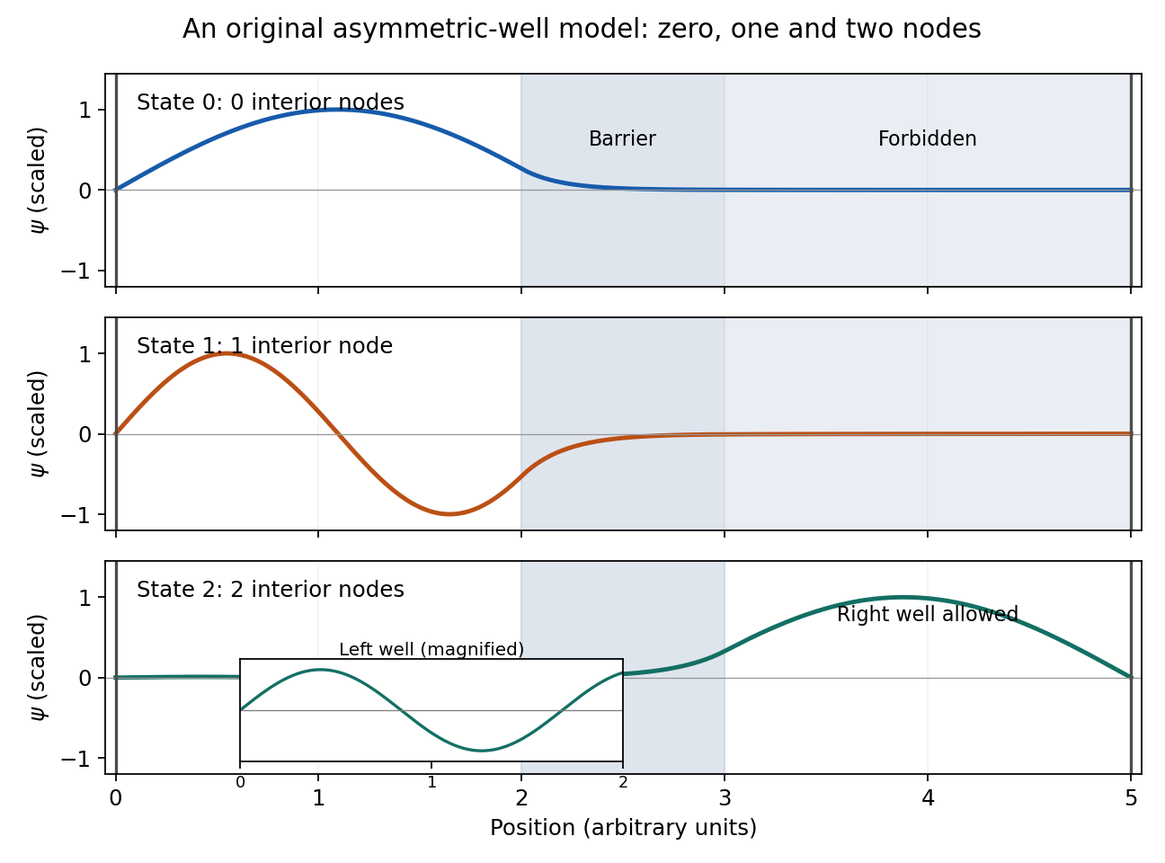
The original illustration solves an explicitly chosen model with the same ordering of allowed and forbidden regions. Its numerical parameters and detailed node positions are illustrative.

Assuming independent Gaussian measurement errors with the quoted standard deviations, use the inverse-variance weighted mean:Here ${\sum }_i{w}_i=0.654514$ and ${\sum }_i{w}_i{x}_i=65.805556$, givingThe consistency statistic is ${\chi }^2=4.45$ for four degrees of freedom, so there is no evident excess scatter requiring error rescaling. A shared systematic error would require a covariance matrix and would not be reduced by this averaging rule.

A small constant input can repeatedly produce the same analogue-to-digital converter code, so averaging those codes cannot reveal its position within a conversion interval. dither makes adjacent codes toggle; their relative frequencies then encode changes smaller than one conversion step. With adequate oversampling, low-pass filtering and averaging reduce the added, sufficiently uncorrelated noise while retaining the slow signal.

For independent sample errors, the averaged standard deviation scales as $N^{-1/2}$; ideally four times as many samples gain about one effective bit. For example a constant input $0.2\Delta$ rounded to levels separated by $\Delta$ would always return zero. Adding uniform dither on $[-\Delta /2,\Delta /2]$ gives output $\Delta$ with probability $0.2$ and zero otherwise: the expected average is $0.2\Delta$, with error $0.4\Delta /\sqrt{N}$. The benefit concerns the filtered estimate, not a more accurate individual conversion. Excessive dither wastes range, and averaging does not correct calibration bias, correlated drift or arbitrary converter nonlinearity.^[ref]