Past exam of the physics A course of the University of Cambridge / 2011 / Paper 2 / Section D / D12

Bayes' theorem updates a parameter distribution using measured data:The likelihood describes the measurement process, the prior distribution encodes information before the present data, and the denominator normalizes the posterior distribution. Include instrumental noise and known selection effects in the likelihood. nuisance parameters, such as an uncertain background, should be jointly inferred and marginalized, rather than silently fixed.

For $n$ independent readings with a Gaussian distribution with known common variance ${\sigma }^2$ and prior distribution $\theta \sim N({\mu }_0,{\tau }_0^2)$, completing the square givesThe posterior distribution is $N({\mu }_n,{\tau }_n^2)$: prior distribution and data contribute in proportion to precision. A broad prior distribution recovers the usual estimate $\bar{x}$ with standard deviation $\sigma /\sqrt{n}$. Report a posterior distribution estimate and credible interval, specify the prior distribution, and examine sensitivity when the data are weak. A credible interval is a posterior distribution probability statement about the parameter conditional on the model; it is not defined by the repeated-sampling coverage of a confidence interval.

Uniform samples at $t_n=n/f_s$ cannot distinguish frequencies separated by integer multiples of $f_s$:For a real cosine, opposite frequencies also coincide. Thus an unknown high-frequency component can appear in the sampled record at its folded frequency $f_{\mathrm{alias}}\in [0,f_s/2]$. For example, 2 Hz and 8 Hz cosines give identical samples at 10 samples per second. This ambiguity is aliasing, rather than uniform quantization error.

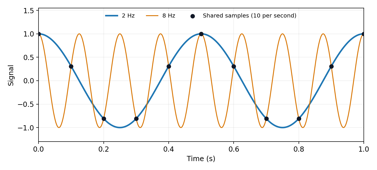
The Nyquist–Shannon sampling theorem permits reconstruction of an ideally bandlimited function of bandwidth $B$ when $f_s>2B$. Use an analogue anti-aliasing filter before conversion and allow a transition band between the desired passband and the frequencies that fold into it. Sampling faster relaxes the filter requirement. Digital filtering after undersampling cannot separate already identical sample sequences. Finite observation time, clock jitter, noise and imperfect filter rejection impose further practical limits.

Identify the physical coupling that causes a systematic error and change the apparatus so that it can be measured or cancelled. measurement calibration against known reference standards at several points reveals zero and gain errors; blanks and background runs measure additive contributions. Carry uncertainties of the standards and fitted corrections into the final result.

Reversal provides a particularly transparent test. If $D_{+}=S+b$ and $D_{-}=-S+b$, the combination $(D_{+}-D_{-})/2$ isolates $S$ while $(D_{+}+D_{-})/2$ measures the measurement zero offset. Interleave and repeat the reversals so drift can be detected. The cancellation assumes a stable measurement zero offset and a genuinely odd signal; a common gain error remains. null measurements and bridge comparisons can reduce dependence on detector gain. Swapping sensors or leads exposes asymmetry; checking alignment, shielding, grounding and temperature control tests specific unwanted couplings. Varying signal amplitude or measurement frequency can reveal heating, nonlinear response or pickup.

Use independent measurement principles where possible, and test the predicted response to each deliberate change. Repeated readings alone do not remove a fixed systematic error. Correct identified significant effects and retain uncertainty for imperfectly known corrections; complete elimination cannot generally be demonstrated. Type A and Type B classify how uncertainty is evaluated, rather than simply meaning random measurement errors and systematic errors.^[ref]