Original paper: FOI release, physical PDF pages 21–27, printed pages 1–7. The solutions include every optional question and note topic.
For a normalizable state take . inverse construction of a quantum potential gives . differentiation yields , so the chosen potential energy zero fixes . ThusThis energy lies above the negative minima of the potential energy; its zero value does not mean zero kinetic energy. The nodeless eigenfunction is the ground state.
The Sturm oscillation theorem gives three nodes of a wavefunction for the fourth bound state. reflection symmetry and nondegeneracy of one-dimensional bound states make it odd: one node of a wavefunction is at the centre, and the other two lie at opposite positions. In each flat allowed region the wavefunction is a sinusoid, with ; its wavelength is shortest in the central, deepest region. Outside the well it decays exponentially, with opposite signs on the two sides. Both and remain continuous at every finite step, as required by wavefunction matching at a finite potential step; only the curvature jumps. In particular, the wavefunction need not vanish at a step.
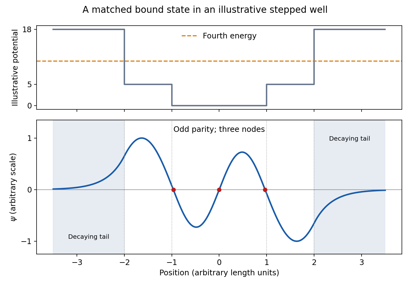
Fourth bound state
. Details. This original wavefunction matching at a finite potential step illustration uses freely chosen well dimensions and energies. It shows the required parity, node count, wavelength ordering and decaying tails; the source drawing supplies no numerical scale from which to fix exact node positions.
The canonical commutation relation is . Applying the commutator product rule on a common operator domain,Equivalently, applying both sides to a twice differentiable test function gives , the same result.
The central estimate is . propagation of uncertainty must include the occurrence of in both numerator and denominator. With angular derivatives measured per radian,Interpreting the two quoted errors as independent standard deviations, convert them to radians before calculatingIf the quoted errors are instead absolute bounds, the first-order worst-case estimate is . Correlated errors add to the variance. Treating and as independent would lose their shared measurement uncertainty.
In the high-resolution quantization approximation, a smooth input distribution varies little across one conversion interval, so rounding to the nearest level gives an approximately uniform quantization error . ThereforeThe input must stay within the analogue-to-digital converter's range. A large standard deviation alone does not guarantee uniform quantization error: an input concentrated exactly on widely separated conversion levels has zero error. Truncation without a half-step correction also has a different mean and root mean square.
For each mode in Cartesian coordinates, and . Consequently the two-dimensional isotropic harmonic oscillator hasThe normalized actions of the creation and annihilation operators areInvert their definitions as and , and similarly for . linear operators belonging to different coordinates commute, so substitution into givesEach term transfers one excitation between the two modes: , and likewise for its adjoint. Thus and, with no explicit time dependence, . This is conservation of angular momentum under planar rotations.
Finally and . HenceThe angular momentum is ; division by performs wavefunction normalization on this state without changing its eigenvalue. It is one excitation of the positive circular mode.
A pure stationary state of a time-independent Hamiltonian operator is . Its probability density and all expectations of time-independent observables are constant. This does not require zero probability current.
For real scalar potential energy and no vector potential, substitute and its complex conjugate into . The potential terms cancel:Thus the probability current is . In a stationary state : flow may circulate without changing the density.
Here only the azimuthal phase contributes an imaginary logarithmic derivative. Since ,There is no radial or polar flow; the azimuthal current is independent of , so its divergence vanishes. The apparent coordinate singularity at cancels in the final expression.
The z-component of orbital angular momentum follows from the moment of the mass current:Indeed . This agrees with acting on the wavefunction.
Write , retaining the printed magnetic moment convention. The displayed two-dimensional matrices are Pauli matrices, and the spin Hamiltonian operator isFor an x-directed field let . The Schrödinger equation gives and . With , these equations yieldEquivalently, . If denotes a positive elementary charge magnitude, a free electron is conventionally assigned a minus sign in its magnetic moment; that alternative reverses the rotation sense. The expressions here consistently use the moment specified in the paper.
Put , . The real part of the off-diagonal coherence vanishes:This also follows from and its zero initial expectation. Individual measurements still give , each with probability .
The populations giveTogether with , this describes Larmor precession of a spin initially perpendicular to the field. The positive angular frequency is ; the sign specifies the rotation sense through . The factor of two between the spinor amplitudes and the measured spin is essential. The model with quantum coherence predicts no decay; spin relaxation or dephasing in a real solid can damp the oscillation.
Put . Substitution of into the time-independent Schrödinger equation, followed by division by and multiplication by , separates the angular dependence:Thus andThe single-valued wavefunction condition, , requires . The regular boundary condition at the origin selects . Accordingly use in the radial ansatz; the printed notation describes the representatives.
For the two-dimensional Coulomb bound state, substitution of with the stipulated radial and energy scales givesThe coefficient of in the power series isThe regular solution otherwise has an exponentially growing contribution at large , incompatible with being normalizable. Termination at degree therefore requiresThe resulting is proportional to a Generalized Laguerre polynomial.
Define , the hydrogenic Rydberg energy for the stipulated mass. The first three distinct two-dimensional energies are , whereas in three dimensions they are . Both series approach zero from below, but the planar ground state is four times more tightly bound. Without spin the respective quantum degeneracies are and ; if individual degenerate states are counted, the second and third planar states already share the first excited energy. This comparison retains the supplied interaction; it does not replace it by the logarithmic electrostatic potential of a genuinely two-dimensional electromagnetic theory.
identical particles have the same intrinsic properties. Exchanging their bookkeeping labels cannot distinguish a physical preparation or change a measurable prediction. This is stronger than merely failing to track classical trajectories. For ordinary bosons and fermions, the many-particle wavefunction has respectively bosonic exchange symmetry or fermionic exchange symmetry under every particle exchange operator, acting on spatial and spin coordinates together. The Spin-statistics theorem connects integer spin to bosons and half-integer spin to fermions; this connection uses relativistic quantum-field assumptions, rather than following from the nonrelativistic Schrödinger equation alone.
For one-particle states satisfying orthonormality, the two alternatives form a quantum superposition:Its probability density contains an exchange interference term, absent from an incoherent mixture of labelled alternatives. The antisymmetric expression vanishes when both one-particle states are identical: one complete one-particle state can contain at most one fermion. This Pauli exclusion principle explains electron shell filling, the electronic Fermi sea and degeneracy pressure. Opposite spins are different one-particle states, so two electrons may share an atomic orbital. Spatially separated wave packets with negligible overlap can often be treated as distinguishable for local measurements; the underlying exchange symmetry remains.
In thermal equilibrium, occupation of a level of energy obeysbosons can accumulate macroscopically in one state, giving Bose-Einstein condensation; fermions instead fill successive states up to the Fermi energy at zero temperature. When occupation is dilute, both expressions reduce to the Maxwell-Boltzmann distribution. The identical-particle classical partition function contains , avoiding spurious entropy from permutations and the Gibbs paradox. Exchange effects become conspicuous when the thermal de Broglie wavelength is comparable to the interparticle spacing.
An operational test is the Hong-Ou-Mandel effect. Down-converted photon pairs enter separate ports of a balanced beam splitter; indistinguishable alternatives for one photon per output cancel. Scanning the relative arrival delay restores coincidences away from overlap. Matching polarization, spectral filtering and spatial alignment controls distinguishability; measuring delayed accidental coincidences controls background. The observed dip tests two-photon interference, and its finite depth must not automatically be interpreted as a failure of bosonic symmetry. The original apparatus varied beam-splitter position and subtracted a separately measured accidental background.[ref]
Measurement of Subpicosecond Time Intervals between Two Photons by Interference by C. K. Hong and others. pp. 2044–2046, Fig. 1, Eq. (2), coincidence-background procedure and Fig. 2
For observables , nonzero obstructs a complete common eigenbasis. In a finite-dimensional system, commuting Hermitian operators can be simultaneously diagonalized; quantum degeneracy may require choosing an appropriate basis inside the degenerate eigenspace. Noncommuting observables can still share particular eigenvectors, so incompatibility is not a claim that every individual state must have nonzero spreads in both quantities.
The Robertson uncertainty relation follows by applying Cauchy-Schwarz inequality to and :In particular gives . These are preparation spreads, not necessarily measurement errors. A zero commutator expectation can make this bound zero even when the linear operators do not commute.
Measurement order can matter: preparing , measuring , then measuring gives both z outcomes with probability when the intermediate result is ignored. A direct z measurement would give certainly. Finally the Heisenberg equation of motion relates commutation to conservation: an observable with no explicit time dependence and is conserved. For unbounded self-adjoint operators these statements require the appropriate common domains; a formal commutator calculation alone need not justify simultaneous spectral measurements.
In a classically forbidden region, the Schrödinger equation has evanescent solutions rather than forcing the wavefunction to vanish. Matching at both sides of a finite barrier permits nonzero transmission. For a broad barrier the WKB approximation giveswhere is a matching prefactor. Transmission is exponentially sensitive to barrier width and height. A single decaying exponential function carries no probability current; the matched scattering solution includes the combination needed for transmitted current. energy is conserved throughout.
In alpha decay, a quasibound alpha particle penetrates the nuclear Coulomb barrier. Multiplying the penetration probability by an assault frequency estimates the decay rate; the strong dependence on alpha energy explains the wide range of lifetimes. In a scanning tunnelling microscope, a voltage drives electron quantum tunnelling between a conducting tip and sample. Approximately , so constant-current feedback resolves changes in gap width, with electronic density of states also affecting the image. Piezoelectric motion, vibration isolation and stable voltage are necessary; a bright feature is not automatically a taller atom. Atomic-scale imaging was demonstrated with a vacuum-tunnelling microscope in the original surface study.[ref]
Surface Studies by Scanning Tunneling Microscopy by Gerd Binnig and others. Abstract and pp. 57–61: atomic-scale steps and surface reconstruction
In a Josephson junction, Cooper pair quantum tunnelling through a weak link gives , allowing supercurrent without an applied voltage and phase-sensitive interference. These are distinct applications of barrier penetration and coupling with quantum coherence, not particles borrowing energy to climb over a barrier.Addition of two spin-one-half angular momenta gives total spin or . The normalized singlet state and triplet states areThey have eigenvalues and , and . The singlet state is antisymmetric under a particle exchange operator, whereas all three triplets have symmetric spin-exchange parity. For two identical electrons the full state must be antisymmetric: a singlet state pairs with a spatial state with symmetric exchange parity, a triplet state with an antisymmetric spatial state. Thus two electrons in the same atomic orbital must form a singlet state.
The identity gives in the singlet state and in the triplet state. Hence an exchange interaction distinguishes their energies, with ordering determined by its coupling sign. The singlet state has perfect opposite-spin correlations along any common measurement axis and is entangled. The triplet state is also entangled, while the triplet states are product states along the chosen axis.
Bayes' theorem updates a parameter distribution using measured data:The likelihood describes the measurement process, the prior distribution encodes information before the present data, and the denominator normalizes the posterior distribution. Include instrumental noise and known selection effects in the likelihood. nuisance parameters, such as an uncertain background, should be jointly inferred and marginalized, rather than silently fixed.
For independent readings with a Gaussian distribution with known common variance and prior distribution , completing the square givesThe posterior distribution is : prior distribution and data contribute in proportion to precision. A broad prior distribution recovers the usual estimate with standard deviation . Report a posterior distribution estimate and credible interval, specify the prior distribution, and examine sensitivity when the data are weak. A credible interval is a posterior distribution probability statement about the parameter conditional on the model; it is not defined by the repeated-sampling coverage of a confidence interval.
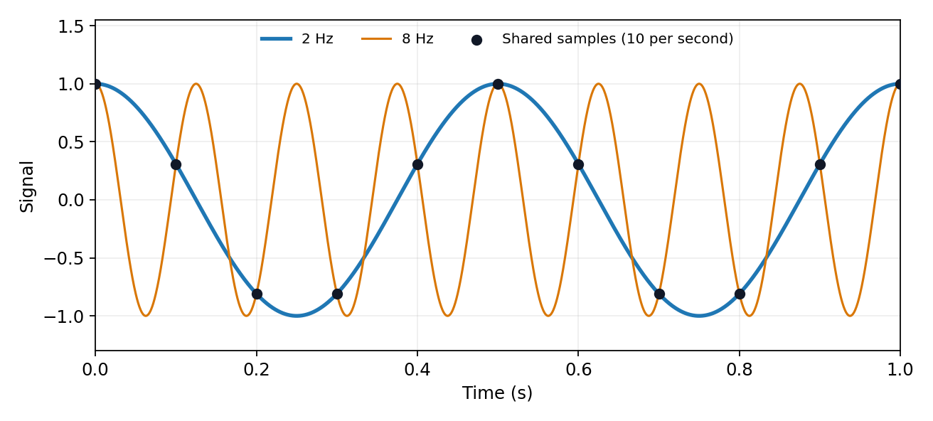
Uniform samples at cannot distinguish frequencies separated by integer multiples of :For a real cosine, opposite frequencies also coincide. Thus an unknown high-frequency component can appear in the sampled record at its folded frequency . For example, 2 Hz and 8 Hz cosines give identical samples at 10 samples per second. This ambiguity is aliasing, rather than uniform quantization error.


The Nyquist–Shannon sampling theorem permits reconstruction of an ideally bandlimited function of bandwidth when . Use an analogue anti-aliasing filter before conversion and allow a transition band between the desired passband and the frequencies that fold into it. Sampling faster relaxes the filter requirement. Digital filtering after undersampling cannot separate already identical sample sequences. Finite observation time, clock jitter, noise and imperfect filter rejection impose further practical limits.
Identify the physical coupling that causes a systematic error and change the apparatus so that it can be measured or cancelled. measurement calibration against known reference standards at several points reveals zero and gain errors; blanks and background runs measure additive contributions. Carry uncertainties of the standards and fitted corrections into the final result.
Reversal provides a particularly transparent test. If and , the combination isolates while measures the measurement zero offset. Interleave and repeat the reversals so drift can be detected. The cancellation assumes a stable measurement zero offset and a genuinely odd signal; a common gain error remains. null measurements and bridge comparisons can reduce dependence on detector gain. Swapping sensors or leads exposes asymmetry; checking alignment, shielding, grounding and temperature control tests specific unwanted couplings. Varying signal amplitude or measurement frequency can reveal heating, nonlinear response or pickup.
Use independent measurement principles where possible, and test the predicted response to each deliberate change. Repeated readings alone do not remove a fixed systematic error. Correct identified significant effects and retain uncertainty for imperfectly known corrections; complete elimination cannot generally be demonstrated. Type A and Type B classify how uncertainty is evaluated, rather than simply meaning random measurement errors and systematic errors.[ref]
An ideal operational amplifier draws no current at either input. With stable operational-amplifier negative feedback in its unsaturated linear range, infinite open-loop gain also gives a virtual short, . The amplifier adjusts its output to enforce that equality; it is not a conducting connection between the inputs. Here , so the ideal summing node is a virtual ground. Kirchhoff's current law gives , hence the ideal gain is .
For the finite-input-resistance inverting amplifier let the inverting-node voltage be , and continue to neglect output impedance. The controlled output and node-current balance areEliminating givesDividing the denominator by gives the requested resistance-sum form. The ideal result follows whenever ; taking alone is insufficient if is small. At finite frequency and the gain are phasor ratios, subject to feedback stability.
With equal resistors and sufficiently large loop gain, . This gives a controlled sign reversal or 180-degree phase inversion, useful for subtraction and opposite-phase signal paths, with amplitude set by a resistor ratio rather than uncertain open-loop gain. The source still sees approximately , so this is not a high-input-impedance voltage follower. For the ideal-input, single-pole model, the noise gain of an operational amplifier is two and the closed-loop bandwidth is approximately half the gain-bandwidth product. Output swing, slew rate and load constraints must also permit linear operation.
A representative bipolar-input 741 amplifier has of order ; the LM741 specification gives a typical at . This is an illustrative device specification, not an identification of an unspecified practical-class part. Other input architectures can have much larger electrical resistance, and finite input capacitance makes the input impedance frequency dependent.[ref]
LM741 Operational Amplifier by Texas Instruments. SNOSC25D, §6.5, p. 5, input-resistance row and its test conditions
The open-loop gain is large and roughly constant at low frequency, then falls as internal poles become important. A dominant-pole approximation isAbove , but before higher poles dominate, , a slope of per decade, with increasing phase lag. The approximate unity-gain frequency is . A 741-class amplifier has typical low-frequency gain about ; this is the open-loop gain, distinct from the feedback-set signal gain. The finite-gain formula at the parent level explains why the closed-loop response eventually rolls off.[ref]
Articles by others on the same topic
There are currently no matching articles.