Past exam of the physics A course of the University of Cambridge / 2011 / Paper 2 / Section D

Bayes' theorem updates a parameter distribution using measured data:The likelihood describes the measurement process, the prior distribution encodes information before the present data, and the denominator normalizes the posterior distribution. Include instrumental noise and known selection effects in the likelihood. nuisance parameters, such as an uncertain background, should be jointly inferred and marginalized, rather than silently fixed.

For $n$ independent readings with a Gaussian distribution with known common variance ${\sigma }^2$ and prior distribution $\theta \sim N({\mu }_0,{\tau }_0^2)$, completing the square givesThe posterior distribution is $N({\mu }_n,{\tau }_n^2)$: prior distribution and data contribute in proportion to precision. A broad prior distribution recovers the usual estimate $\bar{x}$ with standard deviation $\sigma /\sqrt{n}$. Report a posterior distribution estimate and credible interval, specify the prior distribution, and examine sensitivity when the data are weak. A credible interval is a posterior distribution probability statement about the parameter conditional on the model; it is not defined by the repeated-sampling coverage of a confidence interval.

Uniform samples at $t_n=n/f_s$ cannot distinguish frequencies separated by integer multiples of $f_s$:For a real cosine, opposite frequencies also coincide. Thus an unknown high-frequency component can appear in the sampled record at its folded frequency $f_{\mathrm{alias}}\in [0,f_s/2]$. For example, 2 Hz and 8 Hz cosines give identical samples at 10 samples per second. This ambiguity is aliasing, rather than uniform quantization error.

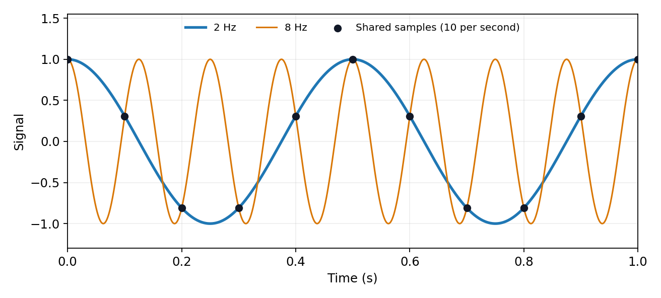
The Nyquist–Shannon sampling theorem permits reconstruction of an ideally bandlimited function of bandwidth $B$ when $f_s>2B$. Use an analogue anti-aliasing filter before conversion and allow a transition band between the desired passband and the frequencies that fold into it. Sampling faster relaxes the filter requirement. Digital filtering after undersampling cannot separate already identical sample sequences. Finite observation time, clock jitter, noise and imperfect filter rejection impose further practical limits.

Identify the physical coupling that causes a systematic error and change the apparatus so that it can be measured or cancelled. measurement calibration against known reference standards at several points reveals zero and gain errors; blanks and background runs measure additive contributions. Carry uncertainties of the standards and fitted corrections into the final result.

Reversal provides a particularly transparent test. If $D_{+}=S+b$ and $D_{-}=-S+b$, the combination $(D_{+}-D_{-})/2$ isolates $S$ while $(D_{+}+D_{-})/2$ measures the measurement zero offset. Interleave and repeat the reversals so drift can be detected. The cancellation assumes a stable measurement zero offset and a genuinely odd signal; a common gain error remains. null measurements and bridge comparisons can reduce dependence on detector gain. Swapping sensors or leads exposes asymmetry; checking alignment, shielding, grounding and temperature control tests specific unwanted couplings. Varying signal amplitude or measurement frequency can reveal heating, nonlinear response or pickup.

Use independent measurement principles where possible, and test the predicted response to each deliberate change. Repeated readings alone do not remove a fixed systematic error. Correct identified significant effects and retain uncertainty for imperfectly known corrections; complete elimination cannot generally be demonstrated. Type A and Type B classify how uncertainty is evaluated, rather than simply meaning random measurement errors and systematic errors.^[ref]

An ideal operational amplifier draws no current at either input. With stable operational-amplifier negative feedback in its unsaturated linear range, infinite open-loop gain also gives a virtual short, $V_{+}=V_{-}$. The amplifier adjusts its output to enforce that equality; it is not a conducting connection between the inputs. Here $V_{+}=0$, so the ideal summing node is a virtual ground. Kirchhoff's current law gives $V_{\mathrm{in}}/R_1=-V_{\mathrm{out}}/R_2$, hence the ideal gain is $-R_2/R_1$.

For the finite-input-resistance inverting amplifier let the inverting-node voltage be $v$, and continue to neglect output impedance. The controlled output and node-current balance areEliminating $v$ givesDividing the denominator by $R_2$ gives the requested resistance-sum form. The ideal result follows whenever $|A|\gg 1+R_2/R_1+R_2/R_{\mathrm{in}}$; taking $R_{\mathrm{in}}\to \infty$ alone is insufficient if $A$ is small. At finite frequency $A$ and the gain are phasor ratios, subject to feedback stability.

With equal resistors and sufficiently large loop gain, $V_{\mathrm{out}}\simeq -V_{\mathrm{in}}$. This gives a controlled sign reversal or 180-degree phase inversion, useful for subtraction and opposite-phase signal paths, with amplitude set by a resistor ratio rather than uncertain open-loop gain. The source still sees approximately $R_1$, so this is not a high-input-impedance voltage follower. For the ideal-input, single-pole model, the noise gain of an operational amplifier is two and the closed-loop bandwidth is approximately half the gain-bandwidth product. Output swing, slew rate and load constraints must also permit linear operation.

A representative bipolar-input 741 amplifier has $R_{\mathrm{in}}$ of order $10^6\Omega$; the LM741 specification gives a typical $2\mathrm{M\Omega }$ at $25^{\circ }\mathrm{C}$. This is an illustrative device specification, not an identification of an unspecified practical-class part. Other input architectures can have much larger electrical resistance, and finite input capacitance makes the input impedance frequency dependent.^[ref]

The open-loop gain is large and roughly constant at low frequency, then falls as internal poles become important. A dominant-pole approximation isAbove $f_p$, but before higher poles dominate, $|A|\propto f^{-1}$, a slope of $-20\mathrm{dB}$ per decade, with increasing phase lag. The approximate unity-gain frequency is $f_T=A_0{f}_p$. A 741-class amplifier has typical low-frequency gain about $2\times 10^5$; this is the open-loop gain, distinct from the feedback-set signal gain. The finite-gain formula at the parent level explains why the closed-loop response eventually rolls off.^[ref]