A nondispersive wave has a linear dispersion relation over the relevant range, so every Fourier transform component has the same phase velocity and group velocity . A wave packet then translates without spreading in an ideal homogeneous lossless medium.
For wave dispersion, depends on frequency or wavenumber. Different components accumulate different phases, and in general the group velocity differs from the phase velocity; variation of group velocity across the spectrum produces spreading of a wave packet. The membrane material can be nondispersive while confinement in a membrane waveguide introduces wave dispersion along its length.
Twice differentiating the proposed normal mode givesIt therefore solves the two-dimensional wave equation precisely whenThe fixed-edge boundary conditions require . The first is automatic, and the second requires . The nonzero normal modes are thereforeThe apparent choice gives identically zero displacement for this sine solution. There are no imposed end conditions in , so is continuous rather than quantized by a second length. For a propagating mode it is real; the plus sign in the stated convention describes propagation in . Each positive integer labels a transverse standing wave across the strip.
For a fixed transverse normal mode, define its cutoff angular frequencyThe longitudinal phase velocity and group velocity, for propagation in , areThus , and . The large longitudinal phase velocity reflects the geometry of the transverse standing wave and does not imply faster transport of energy than the membrane wave speed.
The cutoff frequency of a membrane waveguide for mode isAt cutoff and ; the longitudinal phase velocity has no finite value. Below cutoff,and a bounded field excited at decays as . It is an evanescent wave, rather than a freely propagating mode carrying net time-averaged energy flux down an indefinitely long uniform strip. A finite section can still transmit through coupling of evanescent fields.
The natural interpretation is the fundamental transverse normal mode, . Indeedso only propagates over the main part of the given Gaussian distribution of angular frequencies. Its centre travels atDifferentiate the group velocity with respect to angular frequency:At the centre this is . The one-standard-deviation group velocity spread is consequentlyOver the central travel time the associated spatial shear isEquivalently, use representative components at , for which and . Their separation after isAt a fixed detector away, the corresponding arrival-time difference is .
The paper asks for an estimate of spreading, without specifying a spatial width convention or the initial spectral phase. A Gaussian distribution has no finite full range. Thus is a one-standard-deviation dispersive contribution, whereas about describes the separation of the representatives. Neither is automatically the increase in the packet's original width. For an initially unchirped Gaussian wave packet in the narrow-band approximation, independent initial and dispersive contributions combine as ; a packet with an initial chirp can behave differently. The modal assumption and width convention must accompany the numerical answer.
Different transverse normal modes have different cutoff frequencies and group velocities. A pulse exciting several of them reaches the output in delayed modal components, causing intermodal dispersion, pulse distortion and overlap of successive signals. Their interference also makes the transverse wave intensity pattern depend on propagation distance; irregularities can transfer energy between modes.
Mitigations are to operate between the first and second cutoff frequencies of a membrane waveguide, excite only the desired mode shape with a suitable source, and use smooth uniform boundaries or gradual transitions to reduce mode conversion. Reducing the signal bandwidth keeps its spectrum inside the single-mode interval and reduces group velocity dispersion within the selected mode. Single-mode operation removes intermodal dispersion but does not remove the dispersion derived in part (b).
For the normally incident plane wave, the incident complex amplitude and phase are uniform across the aperture. Treat the field using scalar diffraction, with the aperture represented by its prescribed amplitude transmittance . Let be the distance from the aperture centre to the observation point and let be the transverse direction cosines of that point.
Across an aperture of characteristic size , the Fraunhofer diffraction assumptions are that , so and the obliquity factor is nearly constant, and that the quadratic contribution to the propagation phase is negligible:The remaining path-length dependence is linear:A coherent monochromatic wave and an aperture large enough relative to wavelength for the scalar aperture model complete the usual physical assumptions. The complex amplitude becomeswhere includes the common propagation phase, distance factor and nearly constant obliquity factor. For the central part of a planar screen in the paraxial approximation, and . Small observation angles are useful for that screen-coordinate formula; a general far-field Fourier transform can instead use the exact direction cosines. A lens can also produce this pattern in its focal plane without requiring a physically very distant screen.
The far-field complex amplitude is the two-dimensional Fourier transform of the aperture amplitude transmittance, evaluated at transverse spatial frequencies , . The light intensity is proportional to the squared magnitude of this transform.
Use linearity to add the transforms of simpler aperture components, preserving their relative phases. A translated component acquires a complex exponential factor. Repeated identical openings can be expressed as the convolution of one opening with a sum of Dirac delta functions; the convolution theorem then factors the field into a single-opening transform and an array factor. Multiplying aperture functions instead convolves their transforms. These operations simplify complex apertures without repeatedly evaluating the full diffraction integral. It is the complex amplitudes, rather than their wave intensities, that are added for coherent illumination.
Take the quoted separation to mean adjacent slit centre spacing . For three equal very narrow slits at , the Fraunhofer diffraction complex amplitude in the transverse direction isWith denoting one narrow slit's contribution, the light intensity isThe quotient is interpreted by its limit where both numerator and denominator vanish. At small angles on a screen at , and . Principal interference fringes occur atBetween successive principal maxima there are two zeros, at and . Halfway between them is a smaller maximum , one ninth of a principal peak. The pattern is symmetric about . The positions quoted in millimetres use the paraxial approximation; exactly and .
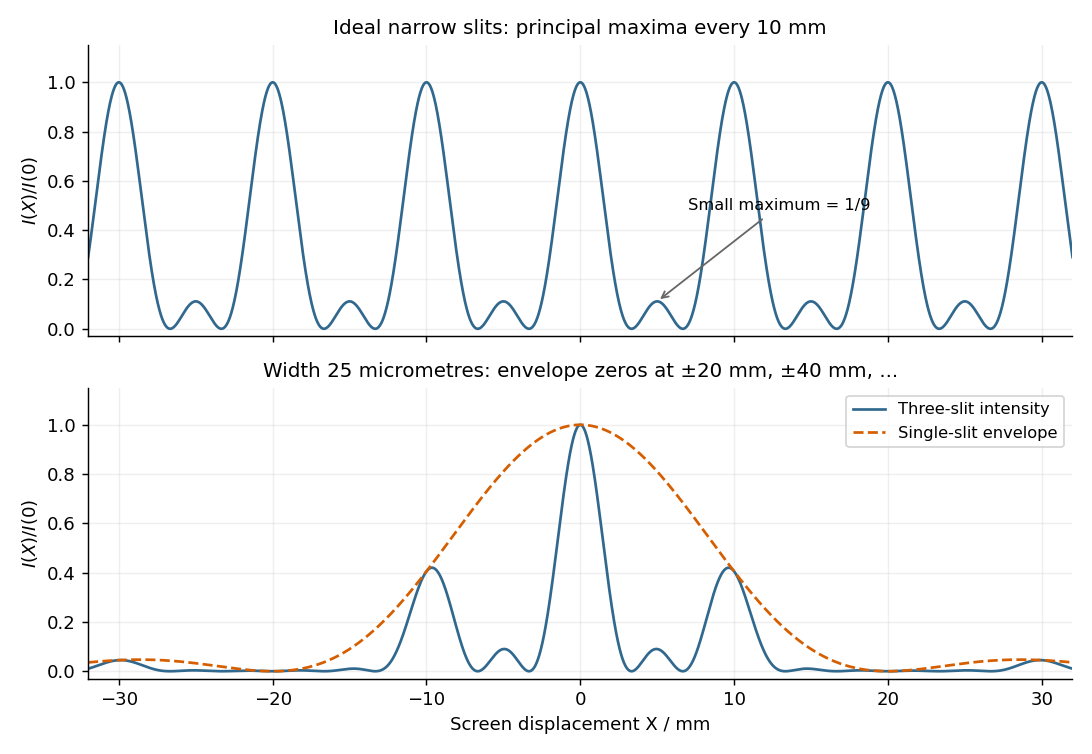
Original calculated Fraunhofer diffraction patterns for three narrow slits and for three finite-width slits
. Details. A slit of width has the single-slit diffraction complex amplitude factor , where . Thus for ,The interference factor keeps the same zeros and the same nominal principal-order positions as in part (i), while the single-slit diffraction wave envelope suppresses off-axis wave intensity. Its zeros areAt nominal principal diffraction orders , the wave envelope factor is . ConsequentlyAll nonzero even principal orders are missing. The central single-slit diffraction maximum extends between the envelope zeros near and includes the central and the principal orders. Because there are only three slits, the maxima of the product can shift slightly from the nominal nonzero-order positions; the quoted values are the exact product at those positions. The lower panel of the figure shows the full product.
Both panels normalize to their own central wave intensity. An absolute comparison would require the unspecified widths and transmitted power of the initially “narrow” slits; the normalized pattern change is fully determined.
For equally spaced illuminated slits, with , summing a geometric series of complex amplitudes givesHere is the one-slit single-slit diffraction wave envelope. The grating equation for principal maxima iswith height and much weaker subsidiary maxima between orders. The first zeros around order are , so the angular distance from a maximum to its first minimum is, for large ,Changing wavelength by moves the same diffraction order byThe Rayleigh criterion places the maximum for one wavelength at the first zero for its neighbour. Equating these separations givesThis is the ideal resolving power of a diffraction grating, for an illuminated and transmitted order with sufficiently narrow source and instrumental broadening. The zeroth order has no wavelength separation and therefore no useful spectral resolving power. The distinction between and the span of the outer slit centres is a small edge convention; the exact state count in the resolving-power formula is .
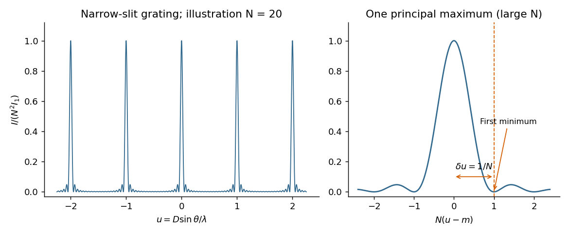


The required resolving power of a diffraction grating isFor illuminated slits, . In orders , the ideal resolvable wavelength differences are respectively , , and . ThusFourth order gives , only a modest margin. It must also exist: for normal incidence the grating equation requires , with needed to avoid an exactly grazing order. The relevant order must transmit appreciable light intensity rather than lie at a single-slit diffraction zero, and the source and detector widths must preserve this resolution.
The original question gives only the slit count, not the line spacing, slit width, usable diffraction order or instrumental broadening. It therefore supports the conditional conclusion “yes in fourth or higher usable order”, but not an unconditional historical claim that this particular instrument resolved the sodium absorption line doublet in its observed configuration.
Articles by others on the same topic
There are currently no matching articles.