Use Fresnel diffraction, since the detector moves along the axis through successive near-field interference extrema. Write for its distance from the opening and for the integration coordinate within the opening. For a uniform incident plane wave, the on-axis complex amplitude, in the paraxial approximation, is proportional toThus the light intensity relative to the incident value isThe Fresnel number is an odd integer at a maximum and an even integer at a minimum. It decreases as the detector moves away. Adjacent extrema therefore differ by one:ConsequentlyAs a check, at and at , so these are indeed a maximum followed by the next minimum. Also , consistent with the paraxial approximation.
The components are in phase quadrature when the axes of the ellipse coincide with the coordinate axes. Since the wave amplitude is one and the wave amplitude is two, the Jones vector must have .
A handedness convention is essential. Adopt the optical convention in which right-handed elliptical polarization rotates clockwise when viewed toward the source, from the positive- side. With the paper's phase convention for complex amplitudes, this givesThe tip follows . In particular,
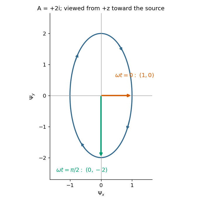
The figure states the viewing direction and shows increasing time. Under the alternative convention that calls rotation from toward right-handed when looking along propagation, the equally consistent answer is and the second vector is . The original paper does not state a handedness convention, so its wording alone cannot select between these labels; the real components and viewing direction remove the ambiguity.
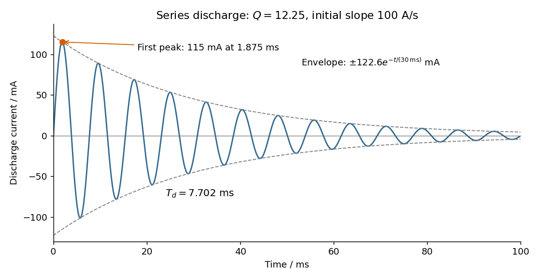
Choose positive electric current in the initial discharge direction, since the source diagram does not label the initial plate polarity or a current arrow. Let be the charge remaining on the initially positive plate, so . Kirchhoff's voltage law for the series RLC circuit givesThe natural angular frequency, damping coefficient and quality factor areSince (equivalently ), this is an underdamped RLC response. With , satisfying the initial conditions givesand differentiating givesThe electric current starts at zero with . Its wave period is , its zeros occur every , and its positive and negative wave envelopes decay with time constant . The first maximum obeys and is at . The electric current tends to zero as the initial capacitor energy is dissipated in the resistor.
Take a p-n junction made from one semiconductor, with the p-type semiconductor on the left and the n-type semiconductor on the right. At thermal equilibrium the chemical potential is horizontal throughout. Before contact the chemical potential lies nearer the valence band on the p side and nearer the conduction band on the n side; after contact the band edges bend to permit one common value.
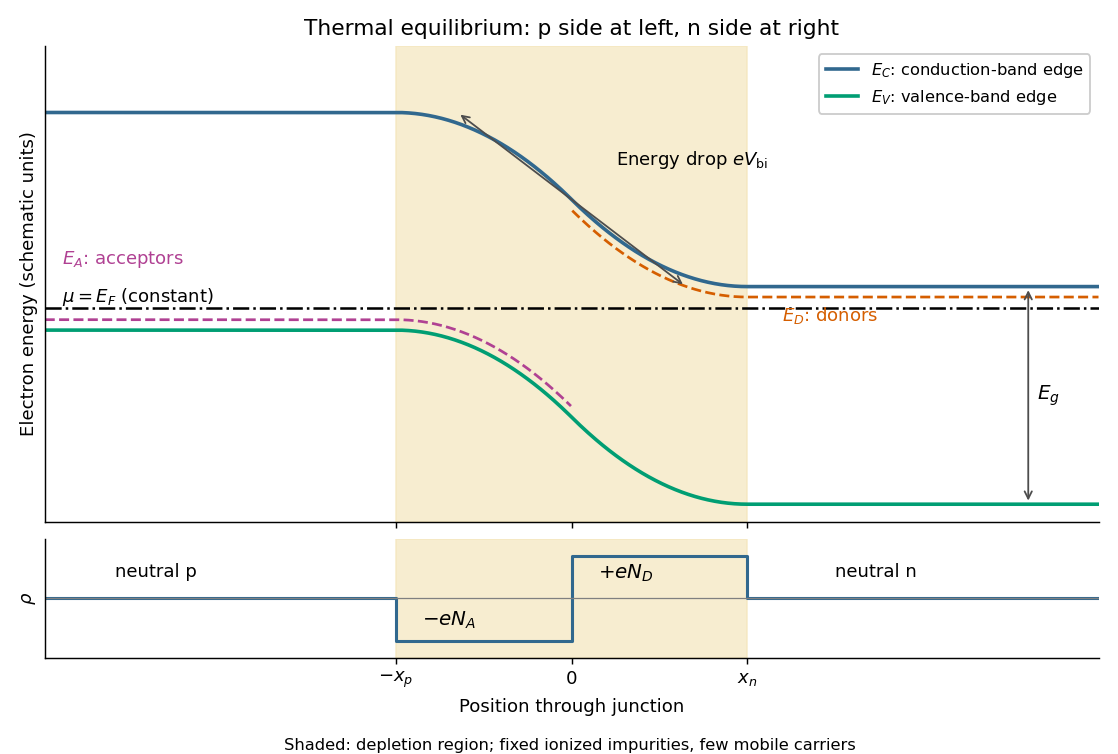
Original equilibrium p-n junction energy band diagram, impurity levels, common chemical potential and depletion region
. Details. In this orientation both the conduction band edge and the valence band edge decrease from p to n by . For a homojunction their separation is constant. The acceptor impurity level lies just above where acceptors are present, and the donor impurity level lies just below where donors are present. These impurity levels follow the local band bending; they do not form one additional horizontal band across the device.
The shaded depletion region has few mobile Electrons or electron holes and contains fixed negative ionized acceptor impurities on the p side and positive ionized donor impurities on the n side. Thus its electric field points from n to p. Its neutral outer regions have negligible electric field, so the band edges become flat there. In the depletion approximation, charge neutrality requires ; the symmetric drawing illustrates rather than assuming that equality is universal. Diffusion and field-driven drift current cancel at equilibrium: no applied voltage does not mean zero internal electric field or zero built-in electric potential difference.
In an ordinary three-dimensional crystalline electrical insulator, heat is carried mainly by phonons. Kinetic theory gives the estimatewhere is heat capacity per unit volume, is a typical sound speed, and is the phonon mean free path. The thermal conductivity has units .
At low temperature, , the Debye model gives . With phonon-phonon collisions frozen out, diffuse scattering at the sample boundaries makes approximately constant, and is nearly constant. HenceAt high temperature, of order or above the Debye temperature, the Dulong-Petit law makes approximately constant. Anharmonic phonon scattering, especially resistive Umklapp scattering, has a collision rate approximately proportional to . Thus andThese two regimes usually give an intermediate maximum of thermal conductivity. The assumptions matter: glassy materials, strong defects or specular boundary reflection can change the low-temperature law; these are not universal laws for every electrical insulator.
A nondispersive wave has a linear dispersion relation over the relevant range, so every Fourier transform component has the same phase velocity and group velocity . A wave packet then translates without spreading in an ideal homogeneous lossless medium.
For wave dispersion, depends on frequency or wavenumber. Different components accumulate different phases, and in general the group velocity differs from the phase velocity; variation of group velocity across the spectrum produces spreading of a wave packet. The membrane material can be nondispersive while confinement in a membrane waveguide introduces wave dispersion along its length.
Twice differentiating the proposed normal mode givesIt therefore solves the two-dimensional wave equation precisely whenThe fixed-edge boundary conditions require . The first is automatic, and the second requires . The nonzero normal modes are thereforeThe apparent choice gives identically zero displacement for this sine solution. There are no imposed end conditions in , so is continuous rather than quantized by a second length. For a propagating mode it is real; the plus sign in the stated convention describes propagation in . Each positive integer labels a transverse standing wave across the strip.
For a fixed transverse normal mode, define its cutoff angular frequencyThe longitudinal phase velocity and group velocity, for propagation in , areThus , and . The large longitudinal phase velocity reflects the geometry of the transverse standing wave and does not imply faster transport of energy than the membrane wave speed.
The cutoff frequency of a membrane waveguide for mode isAt cutoff and ; the longitudinal phase velocity has no finite value. Below cutoff,and a bounded field excited at decays as . It is an evanescent wave, rather than a freely propagating mode carrying net time-averaged energy flux down an indefinitely long uniform strip. A finite section can still transmit through coupling of evanescent fields.
The natural interpretation is the fundamental transverse normal mode, . Indeedso only propagates over the main part of the given Gaussian distribution of angular frequencies. Its centre travels atDifferentiate the group velocity with respect to angular frequency:At the centre this is . The one-standard-deviation group velocity spread is consequentlyOver the central travel time the associated spatial shear isEquivalently, use representative components at , for which and . Their separation after isAt a fixed detector away, the corresponding arrival-time difference is .
The paper asks for an estimate of spreading, without specifying a spatial width convention or the initial spectral phase. A Gaussian distribution has no finite full range. Thus is a one-standard-deviation dispersive contribution, whereas about describes the separation of the representatives. Neither is automatically the increase in the packet's original width. For an initially unchirped Gaussian wave packet in the narrow-band approximation, independent initial and dispersive contributions combine as ; a packet with an initial chirp can behave differently. The modal assumption and width convention must accompany the numerical answer.
Different transverse normal modes have different cutoff frequencies and group velocities. A pulse exciting several of them reaches the output in delayed modal components, causing intermodal dispersion, pulse distortion and overlap of successive signals. Their interference also makes the transverse wave intensity pattern depend on propagation distance; irregularities can transfer energy between modes.
Mitigations are to operate between the first and second cutoff frequencies of a membrane waveguide, excite only the desired mode shape with a suitable source, and use smooth uniform boundaries or gradual transitions to reduce mode conversion. Reducing the signal bandwidth keeps its spectrum inside the single-mode interval and reduces group velocity dispersion within the selected mode. Single-mode operation removes intermodal dispersion but does not remove the dispersion derived in part (b).
For the normally incident plane wave, the incident complex amplitude and phase are uniform across the aperture. Treat the field using scalar diffraction, with the aperture represented by its prescribed amplitude transmittance . Let be the distance from the aperture centre to the observation point and let be the transverse direction cosines of that point.
Across an aperture of characteristic size , the Fraunhofer diffraction assumptions are that , so and the obliquity factor is nearly constant, and that the quadratic contribution to the propagation phase is negligible:The remaining path-length dependence is linear:A coherent monochromatic wave and an aperture large enough relative to wavelength for the scalar aperture model complete the usual physical assumptions. The complex amplitude becomeswhere includes the common propagation phase, distance factor and nearly constant obliquity factor. For the central part of a planar screen in the paraxial approximation, and . Small observation angles are useful for that screen-coordinate formula; a general far-field Fourier transform can instead use the exact direction cosines. A lens can also produce this pattern in its focal plane without requiring a physically very distant screen.
The far-field complex amplitude is the two-dimensional Fourier transform of the aperture amplitude transmittance, evaluated at transverse spatial frequencies , . The light intensity is proportional to the squared magnitude of this transform.
Use linearity to add the transforms of simpler aperture components, preserving their relative phases. A translated component acquires a complex exponential factor. Repeated identical openings can be expressed as the convolution of one opening with a sum of Dirac delta functions; the convolution theorem then factors the field into a single-opening transform and an array factor. Multiplying aperture functions instead convolves their transforms. These operations simplify complex apertures without repeatedly evaluating the full diffraction integral. It is the complex amplitudes, rather than their wave intensities, that are added for coherent illumination.
Take the quoted separation to mean adjacent slit centre spacing . For three equal very narrow slits at , the Fraunhofer diffraction complex amplitude in the transverse direction isWith denoting one narrow slit's contribution, the light intensity isThe quotient is interpreted by its limit where both numerator and denominator vanish. At small angles on a screen at , and . Principal interference fringes occur atBetween successive principal maxima there are two zeros, at and . Halfway between them is a smaller maximum , one ninth of a principal peak. The pattern is symmetric about . The positions quoted in millimetres use the paraxial approximation; exactly and .
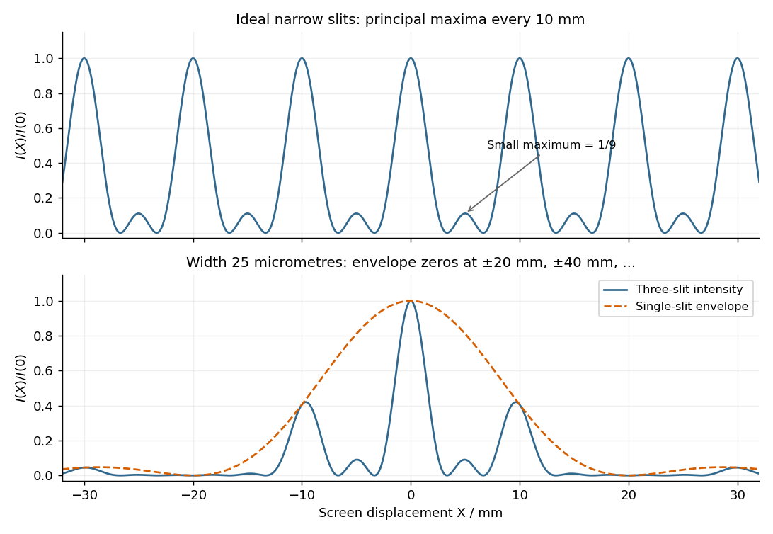
Original calculated Fraunhofer diffraction patterns for three narrow slits and for three finite-width slits
. Details. A slit of width has the single-slit diffraction complex amplitude factor , where . Thus for ,The interference factor keeps the same zeros and the same nominal principal-order positions as in part (i), while the single-slit diffraction wave envelope suppresses off-axis wave intensity. Its zeros areAt nominal principal diffraction orders , the wave envelope factor is . ConsequentlyAll nonzero even principal orders are missing. The central single-slit diffraction maximum extends between the envelope zeros near and includes the central and the principal orders. Because there are only three slits, the maxima of the product can shift slightly from the nominal nonzero-order positions; the quoted values are the exact product at those positions. The lower panel of the figure shows the full product.
Both panels normalize to their own central wave intensity. An absolute comparison would require the unspecified widths and transmitted power of the initially “narrow” slits; the normalized pattern change is fully determined.
For equally spaced illuminated slits, with , summing a geometric series of complex amplitudes givesHere is the one-slit single-slit diffraction wave envelope. The grating equation for principal maxima iswith height and much weaker subsidiary maxima between orders. The first zeros around order are , so the angular distance from a maximum to its first minimum is, for large ,Changing wavelength by moves the same diffraction order byThe Rayleigh criterion places the maximum for one wavelength at the first zero for its neighbour. Equating these separations givesThis is the ideal resolving power of a diffraction grating, for an illuminated and transmitted order with sufficiently narrow source and instrumental broadening. The zeroth order has no wavelength separation and therefore no useful spectral resolving power. The distinction between and the span of the outer slit centres is a small edge convention; the exact state count in the resolving-power formula is .
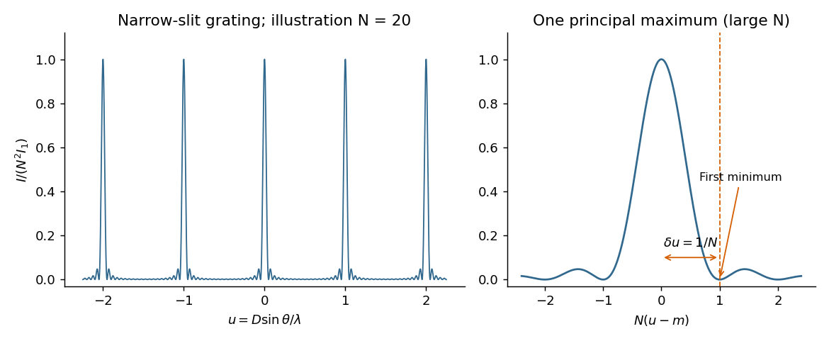


The required resolving power of a diffraction grating isFor illuminated slits, . In orders , the ideal resolvable wavelength differences are respectively , , and . ThusFourth order gives , only a modest margin. It must also exist: for normal incidence the grating equation requires , with needed to avoid an exactly grazing order. The relevant order must transmit appreciable light intensity rather than lie at a single-slit diffraction zero, and the source and detector widths must preserve this resolution.
The original question gives only the slit count, not the line spacing, slit width, usable diffraction order or instrumental broadening. It therefore supports the conditional conclusion “yes in fourth or higher usable order”, but not an unconditional historical claim that this particular instrument resolved the sodium absorption line doublet in its observed configuration.
For a plane wave wavefunction , impose the cyclic or periodic boundary condition . It requiresAdjacent allowed wavenumbers on the full signed axis are spaced by . Ignoring spin, the density of states per unit is consequentlyBoth positive and negative are included in this density. It is not yet the density per unit magnitude , which has an extra factor of two away from zero. In independent dimensions the same periodic boundary conditions give one spatial state per -space cell of measure .
To preserve the convention of part (a), first count one spin species. Define as the number of spatial states in the whole specimen in that energy interval. PutIn one dimension there are intervals near both and , so the one-dimensional free-electron density of states isThus . The factor of two here comes from opposite momenta, not spin. For physical Electrons with two spin states, the spin-summed density of states is . These expressions are continuum approximations away from individual discrete levels.
In two dimensions the density of states in space per spin species is . A annulus of radius and thickness has area . ThereforeThe two-dimensional free-electron density of states is constant in energy, , above the band bottom. Including both spin states gives . Dividing by gives the density per unit physical area, rather than the total specimen's density.
In three dimensions use the -space density of states per spin species and the spherical shell volume :Thus the three-dimensional free-electron density of states grows as . For physical Electrons, including both spin states givesAll three total density of states functions have units when energy is in joules; they count states per energy interval. The paper explicitly suppresses spin in (a) but does not repeat that convention in (b), so giving both conventions avoids a hidden factor-of-two ambiguity. Parts (c)--(f) below use the physical two-spin-state electron gas.
Let and take a specimen of length, area or volume . One monovalent atom per unit cell suppliesElectrons. At zero temperature, the Pauli exclusion principle fills the lowest energy states, with two spin states per spatial wavevector. The occupied region is an interval, disk or ball of radius . Using the -space density of states gives, in one dimension,In two dimensions,In three dimensions,Each Fermi energy follows from the free electron model dispersion relation . The Fermi wavevectors have units and the Fermi energies have units joules for in metres and in kilograms. No numerical lattice spacing is supplied, so numerical energies in electronvolts cannot be uniquely calculated. The spin factor of two is necessary here for actual monovalent crystals; the spinless auxiliary count of part (a) was not an instruction to remove electron spin from these crystals.
For each primitive linear, square or cubic Bravais lattice of spacing , the reciprocal lattice has spacing . The first Brillouin zone is consequently the interval, square or cube with faces at components . The nearest zone boundary is a distance from the centre. The ratios areAll are below one: the ideal free-electron Fermi surface lies wholly inside the first Brillouin zone. Its nearest approach to the boundary is in three dimensions, where it lies only about short of the nearest face. A lattice-induced band gap at a zone face therefore does not by itself make these half-filled systems insulating in the stated free-electron model. Interactions, structural changes and actual electronic band structure can alter that model prediction.
The length, area and volume of a first Brillouin zone are . The corresponding occupied -space measures areHenceThis is state counting, independent of the interval/disk/ball geometry. One Brillouin zone contains one spatial state per unit cell in a single energy band, and that band can hold two Electrons per cell because of spin. One Electron per cell therefore occupies half of it. The “volume enclosed” is the occupied Fermi sea, not the lower-dimensional area of the Fermi surface itself. Its half-volume does not mean half the distance to the zone boundary in two or three dimensions.
Keep the Electron number fixed, soand . Heating smooths the Fermi-Dirac distribution across the Fermi energy, creating holes below and particles above it. The sign of the low-temperature adjustment of chemical potential follows from the local slope of the density of states.
In one dimension, decreases with energy. At fixed , smoothing removes more Electrons below it than it adds above it, so initially rises. In three dimensions, increases, so falls. In two dimensions the constant density of states makes the leading changes cancel, so stays extremely close to in the degenerate regime.
For quantitative checks, a Sommerfeld expansion gives, for ,For a constant two-dimensional density of states above an unbounded parabolic band bottom, the number integral can be done exactly:soIt actually decreases, but its low-temperature correction is exponentially small rather than quadratic. “Constant in two dimensions” is therefore a low-temperature approximation, not an exact statement for every .
The one-dimensional rise is also only an initial trend. In the high-temperature Maxwell-Boltzmann distribution limit, the ideal -dimensional electron gas has , where and is the thermal de Broglie wavelength. It eventually becomes negative and decreases in every dimension. The one-dimensional chemical potential thus passes through a maximum. This high-temperature statement refers to the stipulated unbounded free-electron dispersion relation, not a claim that a real finite-width crystal band remains parabolic indefinitely.
A mass on a spring of stiffness , subject to linear viscous damping and a sinusoidal drive, obeys the forced harmonic oscillator equationHere is displacement, has units , and is a force in newtons. A series RLC circuit is an electrical analogue, with , , and .
- For underdamping, , the motion is , where . The amplitude decays on time and the frequency is reduced from its undamped value.
- At critical damping, , the repeated root gives . This marks the boundary between oscillatory and nonoscillatory relaxation; it is the usual fastest settling without oscillation for a release from rest.
- For overdamping, , with both roots real and negative. At large damping the slow root approaches , so increasing the resistance to motion can slow equilibration.
The constants are set by initial position and velocity. The mechanical energy and its rate of change in free motion areFor weak damping, the cycle-averaged energy decays approximately as . The quality factor is ; for it equals times stored energy divided by the loss per cycle. Logarithmic decrement of successive free-decay peaks determines experimentally.
For driven motion the complete answer is the decaying free transient plus a steady response at the driving angular frequency:At low frequency, and the displacement is nearly in phase with the drive. At , the lag is and . At high frequency, and the lag tends to . The displacement resonance maximum lies atonly when . Thus an underdamped oscillator need not have a nonzero-frequency displacement resonance peak.
In the steady state the mean input power equals the mean dissipated power:This absorption peaks exactly at , rather than at . Its half-power points have bandwidth , so for this linear model. For weak damping, a high quality factor therefore means a narrow strong resonance and a long free-decay time. Exactly zero damping at resonant driving has no finite steady response: a secular amplitude grows with time.
To determine a crystal structure, scatter probes whose wavelength is comparable to atomic spacings, typically . X-ray diffraction, neutron diffraction and electron diffraction probe periodic order through coherent elastic scattering. With incident and outgoing wavevectors , define . Elastic scattering has and constructive interference occurs when , a reciprocal lattice vector. The equivalent Bragg's law iswhere the detector scattering angle is , not . Peak positions reveal plane spacings and the unit cell; systematic absent reflections constrain centring and the atomic basis.
For X-ray diffraction, a laboratory tube or a synchrotron supplies a collimated beam. In a monochromatic single-crystal experiment a goniometer rotates the specimen and an area detector records reflection positions and integrated wave intensities. A powder experiment uses many randomly oriented crystallites; the reflections form cones recorded as rings or peaks versus , permitting indexing and determination of lattice constants without selecting one crystallite. For a cubic cell, for example, . The white-beam Laue method is especially useful for crystal orientation.
The crystal basis structure factor isafter geometric and thermal corrections, including the Debye–Waller factor. For X-rays, describes scattering from the atomic electron density. Thus positions provide lattice geometry while relative wave intensities constrain atomic positions and species. Wave intensities do not directly give the phases of : structure refinement or other constraints must address the phase problem.
Neutron diffraction uses a reactor or spallation source, wavelength selection and a detector bank or time-of-flight detection. Neutrons interact with nuclei through nuclear scattering lengths that vary between elements and isotopes rather than simply with atomic number. This makes them useful for light atoms, isotope contrast and distinguishing some neighbours in the periodic table; their magnetic interaction also probes magnetic order. Electron diffraction in a transmission electron microscope gives strong signals from very small thin crystallites, although strong multiple scattering often complicates quantitative wave intensity analysis. These techniques complement one another.
A phonon dispersion relation requires both momentum and energy transfer, so elastic diffraction alone is insufficient. In coherent inelastic neutron scattering, the measured transfers for phonon creation areHere is the phonon wavevector reduced into a Brillouin zone, and labels an acoustic phonon branch or optical phonon branch. Negative energy transfer corresponds to annihilating an already occupied phonon. For neutrons , so wavelength and energy selection are linked. Typical thermal-neutron energies of a few to tens of millielectronvolts ( electronvolts) are well matched to many lattice vibrations.
A triple-axis spectrometer uses a monochromator crystal to select , the sample as the second scattering axis, and an analyser crystal to select before detection. Rotate these elements and the specimen to hold fixed while scanning ; inelastic peaks locate . Repeat at different along symmetry directions to map the phonon dispersion relation. The dynamic structure factor governs peak weights, including the selection of phonon polarization by the scattering geometry. A time-of-flight spectrometer instead infers outgoing neutron energy from travel time over a known flight path and records many directions simultaneously.
Inelastic X-ray scattering can also resolve phonons when very high energy resolution is available. Optical Raman scattering and Brillouin scattering measure vibrations near the zone centre because photon momentum transfers are small compared with a typical reciprocal lattice spacing; they complement, rather than generally map the entire zone like, momentum-resolved neutron measurements. Ultrasound measurements give the long-wavelength sound speed, the initial slope of an acoustic phonon branch.
Articles by others on the same topic
There are currently no matching articles.