Past exam of the physics of atmospheres and oceans course of the University of Oxford / 2022 / 5

The constants $R_a,R_b,R_d$ are effective reservoir capacities: stored carbon dioxide mass anomaly per unit effective concentration anomaly, in GtCO${}_2$ per ppmv. Only $C_a$ is a literal atmospheric mole fraction; $C_b,C_d$ are scaled reservoir variables chosen to share its equilibrium value. The exchange coefficients $r,s$ are conductances, in GtCO${}_2$ per ppmv per year: $r(C_a-C_b)$ is transfer from the atmosphere to the fast reservoir and $s(C_b-C_d)$ transfer from that reservoir to the deep ocean. They are not by themselves inverse times; division by a reservoir capacity gives an inverse-time rate.

Hydrostatic balance estimates total atmospheric mass as $M_{\mathrm{air}}=4\pi R_E^2\bar{p}/g$. One ppmv of a dilute ideal gas is a mole fraction $10^{-6}$, so, with dry-air molar mass $M_{\mathrm{mol},\mathrm{air}}\simeq 28.97$ g/mol and carbon dioxide molar mass $44.01$ g/mol,The final factor converts kilograms to gigatonnes. This is carbon dioxide mass, not the smaller carbon mass.

For the linear three-reservoir carbon model, with concentrations as a column vector, the linear ordinary differential equation isA homogeneous normal mode has $\mathbf{x}=\mathbf{v}{e}^{\lambda t}$, where $J\mathbf{v}=\lambda \mathbf{v}$. For negative real eigenvalues the e-folding relaxation time is $\tau =-1/\lambda$. The row sums vanish, so ${\mathbf{v}}_3=(1,1,1{)}^T$ has ${\lambda }_3=0$ andEqual effective concentrations generate no exchange. Summing the reservoir budgets givesThus injected carbon dioxide is conserved after emissions cease: the model redistributes it but contains no permanent removal. The zero normal mode records this conserved excess mass, rather than a long but finite decay.

To check the other normal modes are damped, set $D=\mathrm{diag}(R_a,R_b,R_d)$ and $L=-DJ$. ThenThe similarity transformation $D^{1/2}J{D}^{-1/2}=-D^{-1/2}L{D}^{-1/2}$ is a symmetric negative-semidefinite matrix with a one-dimensional kernel, so the remaining two eigenvalues are strictly negative.

Define the two concentration differences $u=C_a-C_b$ and $v=C_b-C_d$. For zero emissions and $R_a=R_b=R$, their ordinary differential equation isWriting the positive decay rates as ${\mu }_i=1/{\tau }_i$, their characteristic equation isConsequentlyFor $r\gg s$, the first normal mode rapidly equalizes the fast reservoirs, giving ${\mu }_1\simeq 2r/R$. The slower evolution treats them as a combined capacity $2R$ exchanging with $R_d$, giving ${\mu }_2\simeq s[1/(2R)+1/R_d]$. ThereforeThe timescale ratio is ${\tau }_2/{\tau }_1\simeq 4r/s\gg 1$ in the joint limit. Since the conserved normal mode has ${\tau }_3=\infty$, the hierarchy is ${\tau }_1\ll {\tau }_2\ll {\tau }_3$.

Here $R=7.8$, $R_d=78$, $r=0.4$, and $s=0.04$, in the stated reservoir units. The exact characteristic coefficients are $P=0.10820513{\mathrm{yr}}^{-1}$ and $Q=0.000315582{\mathrm{yr}}^{-2}$, givingThe leading separation estimates give $9.75$ yr and $325$ yr if finite $R_d$ is retained, or $390$ yr if $R_d/R$ is also sent to infinity. Thus ${\tau }_1\ll 100\mathrm{yr}<{\tau }_2$; a ratio of ten warrants using the exact values for the requested sketch.

Assume initially zero anomalies in all reservoirs. The atmospheric impulse response, obtained by decomposing $e^{Jt}$ into the three normal modes, iswith $w_0=1/93.6=0.01068376$, $w_1=0.06087812$, and $w_2=0.05664324$, in ppmv/GtCO${}_2$. The checks $w_0+w_1+w_2=1/R_a$ and $w_1/{\tau }_1+w_2/{\tau }_2=r/R_a^2$ fix the instantaneous injection response and its initial decay.

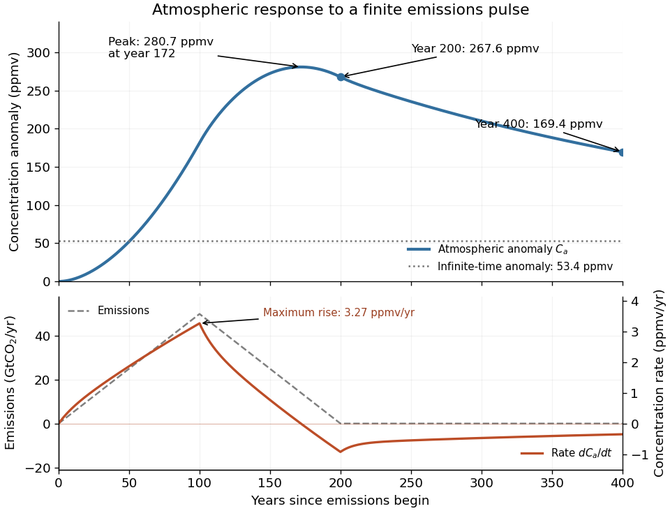
The concentration is the convolution $C_a(t)={\int }_0^{t}G(t-t^{\prime })E(t^{\prime })d{t}^{\prime }$. To evaluate it transparently, define $H_0(q)=q^2/2$ for $q>0$, andsetting every $H_i(q)=0$ when $q\le 0$. Expressing the triangular emission history as $E(t)=0.5[t_{+}-2(t-100{)}_{+}+(t-200{)}_{+}]$ givesHere times are in years and $0.5$ has the corresponding emission-ramp units. Differentiating or evaluating the convolution givesThe maximum concentration occurs earlier than the end of emissions, at approximately year $172$, with $C_a\simeq 280.7$ ppmv. Initially there is a short adjustment over ${\tau }_1$; the curve then rises, turns over as emissions fall, and continues declining after year 200 as the deep ocean takes up carbon dioxide.

The total emitted mass is the area of the emission triangle, $\frac{1}{2}(200)(50)=5000$ GtCO${}_2$. All reservoirs eventually share one concentration, so conservation of mass gives