Carbon-14 has six protons and eight neutrons. Atmospheric production is dominated by using secondary cosmic ray neutrons. It undergoes beta-minus decay to nitrogen-14, with a physical half-life of approximately years.
A layered material with guest species inserted between graphite sheets. Alkali-metal guests can donate electron density to graphitic bands, altering carrier concentration, spacing and scattering.
A potassium graphite intercalation compound, with KC-eight a common stage-one composition. Charge transfer from potassium to the graphitic pi system can enhance electrical conductivity.
Graphene is a single layer of carbon chemical atoms arranged in a honeycomb lattice. A nearby gate can select predominantly electron or electron hole conduction, as demonstrated by the graphene exfoliation and field-effect experiments.[ref]
Electric Field Effect in Atomically Thin Carbon Films by Konstantin Novoselov and others. pp.1–2, mechanically cleaved films, gate and Hall response
A useful question is how geometry changes motion. The nearest-neighbour model of graphene starts with three equivalent bonds from each site and two sites per primitive cell. Interference between those three hopping paths makes two energy bands meet; near their meeting, energy grows linearly with distance in wave vector. The resulting Dirac cones explain why an atomic sheet can imitate one aspect of a relativistic particle while remaining an ordinary material with contacts, defects and boundaries.
The local energy difference between the conduction and valence bands along the boundary of the first Brillouin zone. In a nearest-neighbour model it vanishes at the corner valleys and reaches at edge midpoints; this angular variation is compatible with a globally gapless material.
Separating a layered material into dispersed thin flakes by mechanical processing in a liquid. For graphite, liquid choice, shear or sonication, classification and recovery jointly control the graphene flake distribution. Preserving the lattice does not guarantee a high monolayer yield or a clean final electrode.[ref]
High-yield production of graphene by liquid-phase exfoliation of graphite by Yenny Hernandez and others. 2008, preparation and characterization
graphene oxide that has undergone partial removal of oxygen-containing groups; residual functional groups and lattice defects remain.
Two coupled graphene layers. Their electronic bands depend on relative stacking and external electrostatic conditions, rather than on layer count alone.
Bilayer graphene with a relative rotation between the layers. Hybridization of displaced Dirac cones creates angle-dependent bands and optical resonances.
Take a planar honeycomb lattice with two sites per primitive cell and one localized atomic orbital per site. In this explicitly idealized tight-binding model, all three nearest-neighbour hopping matrix elements are , with ; there is no on-site offset or further-neighbour hopping. Ignore electron interactions and treat physical spin as a separate degeneracy. Let the bond length be , and choose the three vectors from an site to its neighbours asThe Bloch state amplitudes on form a two-component vector. A consistent phase convention gives the HamiltonianIts characteristic equation is , giving the two displayed energy bands. The two-component structure comes from the two sites, rather than two values of physical spin. This is a particularly small matrix model in which a crystal's geometry creates an unexpected low-energy law.
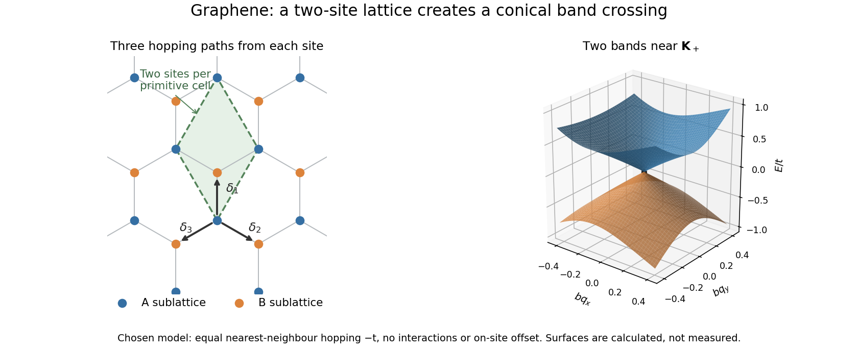
A honeycomb lattice produces two touching electronic bands
. Original nearest-neighbour model with the defined bond vectors. The surface shows the calculated bands near one zero of , with distance in units of inverse bond length and energy in units of the hopping magnitude. These are model energies, not measured band data. Source. Details.Historically, Philip Russell Wallace used a tight-binding model to investigate the electronic band structure of graphite in 1947. The material in that paper was layered graphite; the single-sheet model here isolates one simpler part of the problem.[ref]
The Band Theory of Graphite by Philip Russell Wallace. Publisher abstract: tight-binding bands and Brillouin zones of graphite; published 1 May 1947
At either displayed wave vector, the three complex hopping amplitudes add to zero: . Therefore the energy bands touch. There are two inequivalent electronic valleys; other equivalent corners are related by reciprocal-lattice translations. Setting and retaining first-order terms giveswhere are Pauli matrices. For example, at , . The matrix has the form of a massless two-dimensional Dirac Hamiltonian. Here is a material-model velocity, rather than the vacuum speed of light; this description does not change an electron's vacuum rest mass. It describes the dispersion relation of electronic excitations near a band crossing.
At and positive energy, a normalized eigenvector for is . Its Pauli matrix expectation values give the displayed direction. This pseudospin records the relative amplitudes and phase on the two sublattices. Real spin supplies another label; confusing these two labels would double-count states and misinterpret the two-band Hamiltonian.
Assume zero temperature, the linear Dirac cone, and both real-spin states and both electronic valleys. Define as excess electron number per unit area, negative for an excess of electron holes, relative to neutrality. A filled circular region of radius in wave vector space containsThus the excess carrier density grows quadratically with the Fermi energy, unlike the constant density of states of a parabolic two-dimensional band. Differentiating gives the positive density of states per unit area, . Both the geometry of occupied states and the fourfold degeneracy matter to the coefficient.
A massless-cone description permits a nonzero cyclotron effective mass. For a circular constant-energy contour of area , the semiclassical definition givesThe vanishing mass parameter in a Dirac Hamiltonian and the finite cyclotron response away from neutrality are different statements. This makes the temperature dependence of Shubnikov-de Haas oscillations a useful test of the dispersion rather than a measurement of an electron's vacuum rest mass.
Andre Geim, Konstantin Novoselov and collaborators mechanically cleaved graphite, identified thin flakes, and fabricated multi-terminal Hall bars on oxidized silicon. A substrate gate changed the carrier density; longitudinal electrical resistance and the Hall coefficient supplied different checks. The 2004 report included one-, two- and three-layer devices and described a few-layer semimetal interpretation. Layer identification and electrical control were separate experimental achievements.[ref]
Electric Field Effect in Atomically Thin Carbon Films by Konstantin Novoselov and others. pp.1–2 and Figs.1–2: preparation, thickness selection and electrical measurements
The 2005 monolayer study used an optical microscope, electron microscopy and atomic force microscopy to select monolayers. It then measured Shubnikov-de Haas oscillations as temperature, gate voltage and magnetic field varied. Their damping inferred a density-dependent cyclotron effective mass; comparison with oscillation frequency tested a linear dispersion relation. A comparison with two-layer devices also distinguished their quantum Hall effect sequences. These are complementary tests of the monolayer model, rather than consequences of finding a thin-looking flake alone.[ref]
Two-Dimensional Gas of Massless Dirac Fermions in Graphene by Konstantin Novoselov and others. pp.1–3, Figs.2–4: monolayer selection, oscillation damping and bilayer comparison
Consider an ideal uniform graphene sheet connected to an electron reservoir, with an insulated gate. Let be geometric capacitance per unit area, the elementary charge, and the neutral-point offset. Neglect temperature, trapped electric charge and spatial inhomogeneity. A change in gate voltage pays for both the electrostatic potential drop, , and the change in the sheet's Fermi energy, . Here is measured relative to the band crossing; it is negative for excess electron holes.
Combine this relation with the carrier density in a graphene cone. Write , measured in volts, , and . ThenThe positive root is unique because is strictly increasing for . The often useful geometric approximation neglects the Fermi energy term. It overestimates in this model, especially near neutrality where relatively few states are available.
For a deliberately chosen model with , , and , the formulas give and . The purely geometric value would be . These are chosen-model predictions, not measurements of the historical devices. Numerical conversion uses the exact Planck constant and elementary charge.[ref]
Fundamental Physical Constants — Complete Listing by National Institute of Standards and Technology and others. Exact h and e entries; material parameters in this example are stipulated
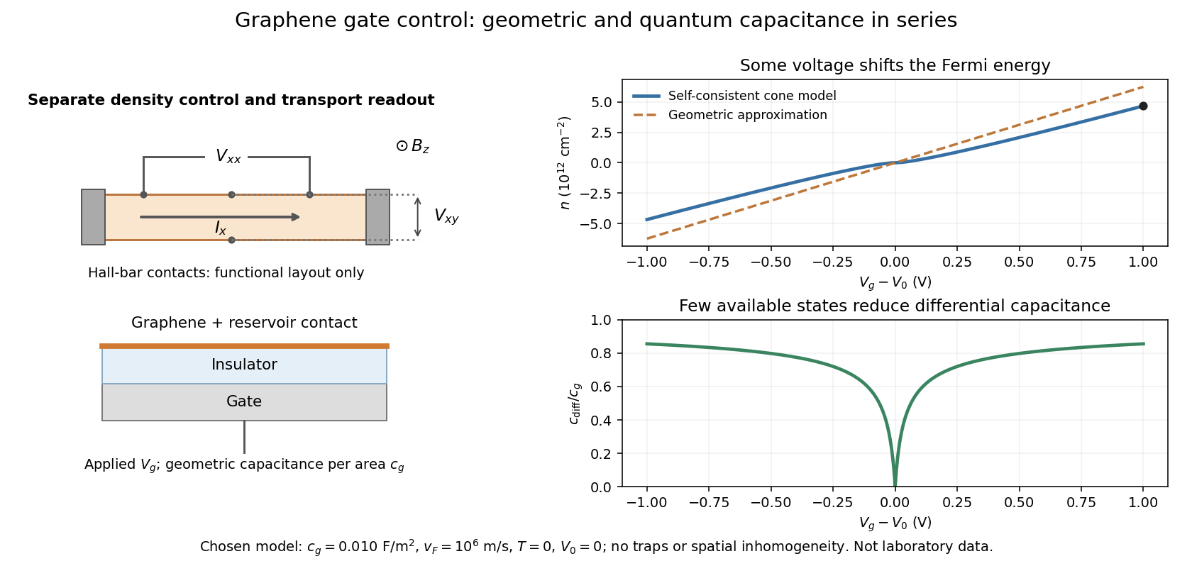
The quantum capacitance per unit area is . Differentiating the gate equation givesThus the available electronic states act as a second contribution in series with geometric capacitance. At exact neutrality the ideal zero-temperature model has ; actual finite-temperature or spatially nonuniform samples need a broader description. A capacitance measurement can therefore probe the density of states, rather than geometry alone.
A strength estimate formed by dividing the maximum axial force supported by load-bearing carbon bonds by the tube mass per length. Equal bond loading and a defect-free, fully participating shell are strong assumptions; network fibres can be limited by intertube shear and sliding.
A dense population of approximately aligned carbon nanotubes growing from a support. Collective crowding can favor alignment even when the support does not epitaxially select every tube orientation.
A plot of optical transition energies against carbon nanotube diameter, usually organized by wrapping indices and electronic type. It relates optical and resonant Raman spectroscopy observations to nanotube structure.
A carbon nanotube comprising several nested graphitic walls. Each shell can have its own wrapping indices; their difference alone is not a structural defect.
An area-based estimate treating each nanotube shell as a graphene cylinder. For graphene atomic area density and shell radii , the carbon count per axial length is . Defects and partial shells change the estimate.
A carbon nanotube comprising one rolled graphene wall. The wrapping indices determine its allowed circumferential electronic wave vectors and therefore its metallic or semiconducting band structure.
An enriched population selected by wrapping indices or electronic type. Sorting can narrow optical transition distributions or remove metallic leakage paths from semiconductor networks. Purity, yield, residual sorting agents and the processed-device environment remain separate performance variables.
An optical excitation between nanotube electronic subbands, often labelled for prominent axial-polarization transitions. One-dimensional Van Hove singularities enhance the joint density of states, but selection rules, oscillator strengths and strong excitons interactions determine actual absorption peaks. Dielectric environment, bundling, doping and defects can change those peaks.
An approximation that samples the graphene bands on wave vectors satisfying , where is the carbon nanotube chiral vector. It produces one-dimensional subbands and the ideal metallicity criterion ; curvature and interactions can modify its predictions.
Circumferential momentum quantization of a graphene Dirac cone produces nanotube dispersion . Comparing with a massive one-dimensional Dirac Hamiltonian identifies the displayed effective mass and gap . This is an emergent band mass, not a changed vacuum electron rest mass. A quantization line through the valley gives zero mass in the ideal zone-folding model; curvature, strain and interactions can change that idealization.
The graphene translation that becomes a tube circumference when its endpoints are identified. It determines wrapping indices and diameter ; it is perpendicular to the tube axis.
The angle of the wrapping vector from the zigzag direction of graphene. For chiral indices , , ranging from zero for zigzag tubes to 30 degrees for armchair tubes. Together with diameter, it determines the discrete wrapping geometry, but does not alone determine the observed colour of a nanotube suspension.
In ideal nanotube zone folding, a single-walled carbon nanotube with indices satisfying . Circumferential quantization misses the Dirac valleys in graphene, opening a band gap.