Source paper: released examination archive, member
2016/T/a13764w1.pdf. The printed cover dates this examination to 15 June 2017.By independence of random variables, the joint probability density is the product of the two probability density functions of the rate-one exponential distributions:Its values on the boundary are immaterial, because the boundary has zero area.
Use the inverse change of variables for probability densitiesIts absolute Jacobian determinant isThereforeSince , its marginal densities are and . The joint density factorizes as , so and are independent random variables, with uniform on and in the shape-rate convention. This is beta-gamma independence with both shape parameters equal to one.
Put . The independent pair has the same joint distribution as from part (ii), because both first coordinates are uniform and independent of the same sum law. HenceConsequentlyThe rate is one. This multiplication identity is the mechanism behind the exponential invariant law of a random affine recursion.
The answer isIt holds initially by construction. If it holds at step , then is a function of , so it is independent of the fresh inputs . Part (a)(iii) therefore gives . This completes the mathematical induction and identifies the stationary distribution of the recursion.
The two recursions use a synchronous coupling: they receive exactly the same fresh inputs. Subtraction cancels the additive term:The variable is independent of the preceding difference and has expected value . Thus expectation of a product of independent random variables givesBy Markov's inequality, for every ,This proves the requested convergence in probability; in fact the difference has L1 convergence. It is synchronous contraction of a random affine recursion, and the estimate holds for every real .
Every has the same exponential distribution, so for . Part (ii) gives . Applying Slutsky's theorem to yieldsThe limiting probability distribution does not depend on . This is precisely the attraction to the exponential invariant law of a random affine recursion.
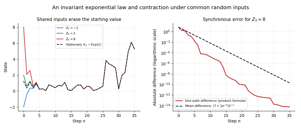
Common random inputs make different initial values approach the same stationary trajectory
. Original simulations of the affine recursion with shared inputs. The right panel compares an exactly propagated path difference with its unconditional expected value; the geometric expectation estimate, rather than the simulation, proves convergence. Details.
The update defines a time-homogeneous Markov process: given its present value, the next value depends only on independent fresh input. Part (b)(i) identifies an invariant law: initializing with the rate-one exponential distribution preserves that distribution at every time. Part (b)(iii) shows convergence of the one-time laws to this invariant law from every deterministic initial value.
For a countable state space, the analogous countable-state Markov chain convergence theorem says that an irreducible Markov chain that is aperiodic and positive recurrent converges to its unique stationary distribution from every initial state. Here the state space is continuous, so that countable-state theorem does not directly supply the proof; the explicit coupling does. The two conclusions have the same equilibrium interpretation.
The moment-generating function of a real random variable isfor real where the expectation is finite. One may regard it as an extended nonnegative function elsewhere. In particular ; finiteness on a neighborhood of zero is the usual hypothesis for recovering moments and using its local expansion.
Differentiating the moment-generating function at zero givesThe second derivative is the second raw moment, so the variance is . The assumed exponential integrability justifies these derivatives.
Integrate against the standard normal density by completing the square:Thus the moment-generating function of a standard normal variable is
Let be real independent and identically distributed random variables with finite expected value and variance . The central limit theorem statesEquivalently, the cumulative distribution functions of these normalized sums converge at every real point to the standard normal distribution function. The theorem itself does not require a finite moment-generating function.
The given expected value and variance imply , and . The Taylor expansion therefore givesSince as , it follows thatThis is the quadratic expansion of a cumulant-generating function for a centered variable of variance one.
Write . By independence of random variables, its moment-generating function isFor each fixed real , the expansion in part (i) yieldsFor the equality is immediate. Exponentiation gives , the moment-generating function of a standard normal variable. The functions are finite on a common neighborhood of zero, so the convergence theorem for moment-generating functions provesThis proves the central limit theorem under the exponential-moment hypothesis of this part.
Use the deterministic weights . Their squared sum and maximum areTo apply the quadratic expansion of a cumulant-generating function rigorously, write , with . Fix and letAll arguments lie in this shrinking interval. ConsequentlyTaking logs of the moment-generating function and using independence of random variables now givesThe case is immediate. Since is the moment-generating function of a normal distribution of variance , the convergence theorem for moment-generating functions givesThis is a weighted central limit theorem with negligible maximum weight. Its limit variance also agrees with the exact value from variance additivity for independent random variables.
A transition matrix defines an irreducible Markov chain if every state is accessible from every other state:Equivalently, all states belong to one communicating class. When , a positive number of steps is necessarily used.
A stationary distribution is a nonnegative row vector with total mass one that is preserved by one transition:In matrix notation, . If the initial state has distribution , so does the state at each later time.
For an irreducible Markov chain on a countable state space, the set has either zero or one element. By uniqueness of stationary distributions for an irreducible countable chain, a stationary probability distribution exists exactly in the positive recurrent case, and thenfor the first return time . The right-hand side fixes every entry, proving uniqueness.
For a finite state space, existence is guaranteed, so there is exactly one. A countably infinite state space can have none: the simple symmetric random walk on the integers is irreducible and null recurrent. Periodicity does not affect this existence-and-uniqueness statement.
The difference process is a Markov chain. If the columns are equal, the next block creates a height difference of one. If the difference is , landing in the taller column increases it to , while landing in the shorter column makes it zero. Therefore its only nonzero transition probabilities areThese probabilities depend only on the present difference, not on the absolute heights or their history. This is the reset-or-increment Markov chain with .
For its stationary distribution, the incoming-flow equations give and for . Normalization uses a geometric series:ThusThe remaining balance equation is also satisfied: the flow into zero is . Every state can reach zero and every positive state can be reached from zero, so it is an irreducible Markov chain. Its invariant probability distribution makes it positive recurrent, and that distribution is unique.
The maximum-height process is not Markov. Starting empty, condition first on the positive-probability history . After two blocks the columns were equal, so after three their difference is one. Hence .
For the history , the first two blocks built one column and the third caught the other column up, leaving equal heights. Hence . Both histories have the same time and present height , but different predictions. This violates the Markov property and illustrates why a function of a Markov chain need not be Markov.
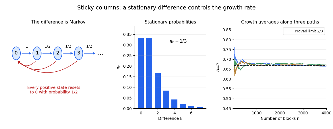

The precise conclusion isTo prove it, observe that the maximum rises exactly when the new height difference is positive:A block landing in a shorter column produces and no rise; every other case raises the maximum and leaves . Starting from , telescoping givesThe difference chain is irreducible and positive recurrent by part (i). Apply the countable-state Markov chain ergodic theorem to the bounded indicator function . Its stationary mean is , giving the asserted almost sure convergence. No aperiodicity assumption is needed for this time average. This establishes the growth rate of two-column sticky deposition.
Articles by others on the same topic
There are currently no matching articles.