Past exam of the topics in applied mathematics course of the University of Oxford / 2011 / A

Write $f(N)=\alpha N^2/(\beta N^2+S)$. Its nonnegative fixed points are $N=0$ and, when ${\alpha }^2\ge 4\beta S$,Indeed a positive fixed point satisfies $\beta N^2-\alpha N+S=0$. The linear stability multiplier isAt a positive fixed point, $\beta N^2+S=\alpha N$, henceFor strict discriminant positivity, $N_{+}$ is attracting and $N_{-}$ repelling; the extinction state is superstable. At equality the positive point has multiplier one. Sinceit attracts from above and repels from below at equality. This is a semistable fixed point, whose one-sided behavior requires the nonlinear calculation.

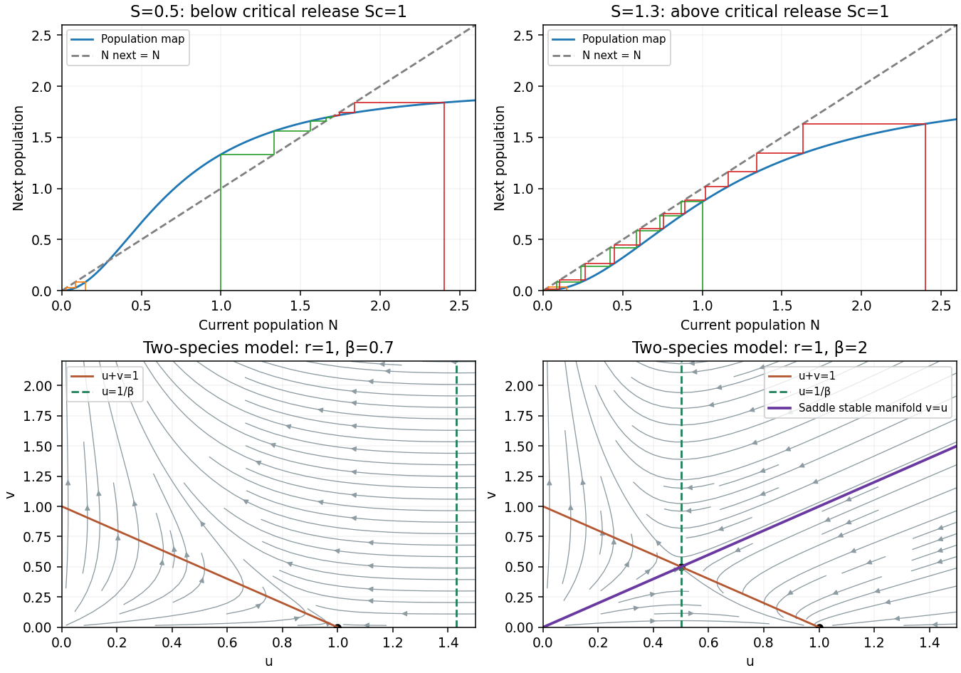
The two positive fixed points merge whenHere $f^{\prime }(N_c)=1$, $f^{\prime \prime }(N_c)\ne 0$, and increasing $S$ decreases $f$, so this is a saddle-node bifurcation of the map. For $S<S_c$, the cobweb descends to zero below $N_{-}$, rises towards $N_{+}$ between the positive fixed points, and descends towards $N_{+}$ above it. Monotonicity of $f$ prevents a trajectory from overshooting across the attracting fixed point. Thus $N_{-}$ is an extinction threshold.

For $S>S_c$, $f(N)<N$ for every $N>0$. The iterates decrease to a nonnegative fixed point, necessarily zero. At $S=S_c$, initial states below $N_c$ tend to zero and those above tend to $N_c$. The sterile-release population threshold therefore combines bistability below the critical release with extinction above it.

The term $ru$ is unrestricted growth of species $u$, and $-r{u}^2$ represents its density-dependent self-limitation, with scaled carrying capacity one. The interaction $-ruv$ suppresses $u$ in the presence of species $v$.

Species $v$ has intrinsic growth $v$ and suppression $-\beta uv$ by $u$. Thus both interspecific effects are harmful: this is a competition model, with no self-limitation term for $v$. Its unbounded growth when $u$ disappears is a consequence of that modeling choice. The parameter $r$ is the growth-time ratio, while $\beta$ measures the effect of $u$ on $v$.

The equilibrium points areThe third is biologically interior only for $\beta >1$, and coincides with $(1,0)$ at $\beta =1$. The Jacobian matrix isAt $(0,0)$ the eigenvalues are $r,1$, so it is a repelling node. At $(1,0)$ they are $-r,1-\beta$, giving a stable node for $\beta >1$ and a saddle for $\beta <1$.

At the interior equilibrium,so coexistence is a saddle. The formal equilibrium with negative $v$ for $\beta <1$ is not a population state; there its trace is negative and determinant positive.

At $\beta =1$ the boundary equilibrium is nonhyperbolic. To determine its behavior into the positive quadrant, put $x=u-1$. A local center manifold has $x=-v+v^2/r+O(v^3)$, so $\dot{v}=v^2+O(v^3)>0$ for small positive $v$. Thus it is unstable to introduction of species $v$, though attracting along the $v=0$ axis. The boundary/interior branches undergo a transcritical bifurcation at this parameter.

The positive quadrant is invariant. The non-axis nullclines are $u+v=1$ and $u=1/\beta$. Below $u+v=1$, $u$ increases; above it, $u$ decreases. To the left of $u=1/\beta$, $v$ increases; to the right, it decreases.

For $\beta >1$, the stable manifold of the interior saddle separates trajectories tending to $(1,0)$ from those for which $u\to 0$ and $v\to \infty$. Exactly on that manifold, the trajectory tends to the saddle. For the illustrated $r=1,\beta =2$, the separating manifold is exactly $v=u$, since the vector field preserves that diagonal.

For $\beta <1$, every strictly positive initial state ultimately has $u\to 0$ and $v\to \infty$. Indeed $\dot{u}\le ru(1-u)$ implies $\mathrm{limsup}u\le 1$, so eventually $1-\beta u$ is bounded below by a positive constant. Then $v$ grows exponentially, forcing $u$ down. At $\beta =1$, a positive $v$ eventually drives $u$ below one; thereafter $v$ increases. A finite positive limit for $v$ would force $u\to 1$, inconsistent with $\dot{u}\to -rv<0$, so the same exclusion outcome holds.

There are no interior periodic orbits: the Bendixson-Dulac criterion with multiplier $1/(uv)$ givesThe phase portraits in the preceding figure show the threshold geometry and the absence of a bounded attracting coexistence state. Initial states on the axes retain the corresponding one-species dynamics.

Let $J$ be population flux. For any fixed control volume $V\subseteq \Omega$, mass conservation with local production givesAssume local, isotropic random dispersal, no imposed advection, and constant diffusion coefficient $D$. Fick's first law is $J=-D\nabla u$. The divergence theorem and arbitrariness of $V$ yieldThe coefficient has units length squared per time; $f$ has units population density per time. Smoothness sufficient to pass from the integral balance to the local equation is understood. This is a reaction-diffusion equation.

The travelling-wave reduction of a reaction-diffusion system of Fisher's equation isMultiplying by $U^{\prime }$ and integrating gives $c{\int }_{\mathbb{R}}(U^{\prime }{)}^{2}dz=1/6$, so the decreasing invasion front has $c>0$. The linearization at $U=0$ has spatial eigenvaluesFor $0<c<2$ they are complex: approaching zero spirals in the $(U,U^{\prime })$ plane and changes the sign of $U$, which is inadmissible for a density. Thus $c\ge 2$ is necessary.

It is also sufficient. Write $V=U^{\prime }$ and choose $\ell =(c-\sqrt{c^2-4})/2>0$. The triangleis forward invariant for $U^{\prime }=V$, $V^{\prime }=-cV-U(1-U)$. On $V=0$, $V^{\prime }\le 0$. On $V=-\ell U$,The boundary $U=1$ points left, and the boundary at $U=0$ consists only of the origin. The unstable branch from the saddle $(1,0)$ enters this triangle, where $U$ decreases and remains nonnegative. Its limiting state must have $V=0$ and $U(1-U)=0$; since it has left $U=1$, it tends to $(0,0)$. Therefore a monotone positive front exists for every $c\ge 2$, including the double-root endpoint:This is the Fisher-KPP minimum wave speed, obtained with an explicit invariant-region existence argument.

Set $Y=U^{q/2}$ and $k=2b/q$. The proposed profile with $a,b>0$ givesSubstituting into $U^{\prime \prime }+c{U}^{\prime }+U(1-U^q)=0$ and dividing in the interior by $U(1-Y)$ yieldsEquating the constant and $Y$ coefficients givesHence the exact generalized Fisher front isThe free positive $a$ translates the front. It connects one on the left to zero on the right and is strictly decreasing. At $q=1$, its speed is $5/\sqrt{6}$.

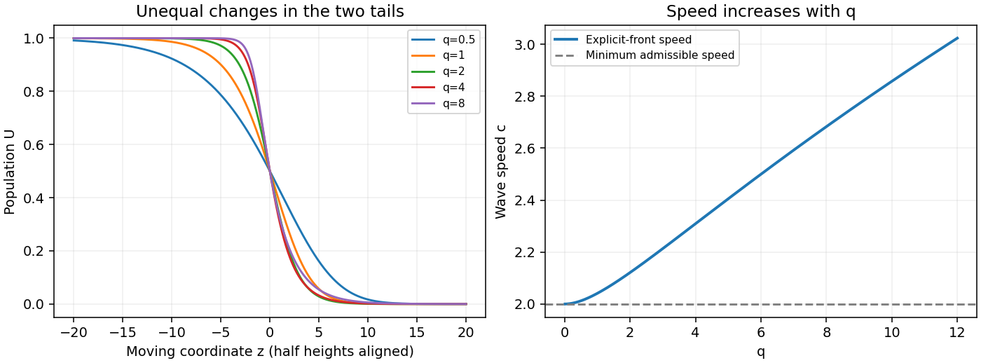
The explicit travelling wave speed increases with $q$:Its two tails change differently. Near the leading empty state, $U\sim a^{-2/q}{e}^{-kz}$ with $k=\sqrt{2/(q+2)}$ decreasing as $q$ grows: that tail lengthens. Near the filled state, $1-U\sim (2a/q)e^{bz}$, with $b=q/\sqrt{2(q+2)}$ increasing: that tail becomes steeper. Thus the change is not a uniform sharpening of the whole profile. For example the half-height slope is $-\frac{k}{2}(1-2^{-q/2})$.

For meaningful comparison, the figure aligns all fronts at $U(0)=1/2$ by choosing $a=2^{q/2}-1$. It displays the speed increase and the unequal changes of the two tails. Since $f^{\prime }(0)=1$ for every $q$, the minimum admissible speed remains two; the explicit family has $c(q)>2$ for $q>0$. The invariant-triangle proof above extends with boundary derivative $U^{q+1}\ge 0$.

Let $r$ be bacterial intrinsic growth rate, $K$ carrying density, $\sigma$ chemical production per bacterial density per time, and $\mu$ chemical decay rate. The bacterial flux iscombining random diffusion with chemotaxis up the chemical gradient. Chemical flux is $J_A=-D_A{A}_x$. The two local balances give the Keller--Segel model with logistic growth:All transport and rate parameters are positive. The production rate is constant per cell, so total production is proportional to $N$.

Choose any positive chemical concentration scale $A_0$ and setAfter dropping hats, substitution giveswhereFor explicit dimensional checks, write bacterial-density and chemical-concentration units as $\mathsf{N},\mathsf{A}$. Then $[D_N]=[D_A]=L^2/T$, $[r]=[\mu ]=T^{-1}$, $[\bar{\chi }]=L^2/(T\mathsf{A})$ and $[\sigma ]=\mathsf{A}/(T\mathsf{N})$. Since $[K]=\mathsf{N}$ and $[A_0]=\mathsf{A}$, each displayed ratio has unit one. The new spatial domain is $[0,1]$.

The nonzero homogeneous equilibrium is $\boxed{n_{\ast }=1,a_{\ast }=\alpha /\beta }$. Without transport its Jacobian matrix iswith negative eigenvalues $-1,-\beta$.

Zero chemical flux gives $a_x=0$ at the endpoints; zero bacterial flux then gives $n_x=0$. Linear perturbations therefore have Neumann boundary conditions and modes $\cos (k_{m}x)$, $k_m=m\pi$. For each mode, the amplitude matrix isIts trace is always negative. Its determinant isA mode grows exactly when $\Delta (k_m)<0$. In particular, any nonzero mode is destabilized by sufficiently large $\chi$. For continuously variable $k$, a nonempty unstable band exists precisely whenWriting $C=\alpha \chi -D_a-\beta D_n$, its squared-wavenumber endpoints are $[C\pm \sqrt{C^2-4\beta D_n{D}_a}]/(2D_n{D}_a)$. On the finite interval, at least one allowed $k_m^2$ must lie inside this band. The uniform $m=0$ mode stays stable. This is the chemotactic pattern-instability criterion.

Chemotaxis supplies positive feedback: a local increase in bacterial density produces more attractant, whose gradient draws in more bacteria. Ordinary cell diffusion opposes aggregation. Chemical diffusion spreads the signal and removes very sharp gradients, while decay and logistic growth stabilize the uniform kinetics.

The dispersion relation from the preceding matrix makes the competition quantitative: the positive $D_n{D}_a{k}^4$ term stabilizes sufficiently short wavelengths, whereas the negative chemotactic contribution $-\alpha \chi k^2$ can destabilize intermediate wavelengths. Increasing cell diffusivity or chemical decay raises the attraction threshold. A growing allowed spatial mode produces correlated patterns in cell density and chemical concentration; the eigenvector relation $(\lambda +\beta +D_a{k}^2)\delta a=\alpha \delta n$ puts their peaks in phase for the growing real mode.

This predicts initial pattern formation. Nonlinear saturation and stability of the eventual pattern require the nonlinear equations, beyond the linear instability test.