This is the 12 June 2018 preliminary examination. Questions 1–4 concern functional programming; Questions 5–8 concern algorithm design and analysis of algorithms. Every printed option is answered here. The complete nine-page native paper is preserved in the Oxford examination release, member
a10097w1.pdf; the damaged duplicate rendition is not the source used here.The Haskell definitions below use finite total inputs unless lazy evaluation, strict functions or infinite lazy lists are being discussed. Separate questions use separate namespaces: in particular their
One constructors are unrelated, and the list-conversion function abs in Question 3 is distinct from the numeric Standard Prelude function. Treat alternative definitions of the same function separately. In a module for Question 2, use import Prelude hiding (zip, zipWith); in one for Question 3, use import Prelude hiding (abs, reverse, (++)). Other questions retain the Standard Prelude operations they use.[ref] Costs count constructor, comparison and ordinary arithmetic operations; integer bit costs and evaluating arbitrary element values are separate.Tree is a type constructor, taking the element type parameter a to the algebraic data type Tree a. It is not a value and has no ordinary value-level function type; its kind of a type is * -> *. The other names are data constructors with polymorphic type signatures:One :: a -> Tree a
Two :: Tree a -> Tree a -> Tree aOne constructs a leaf-labelled binary tree with one leaf; Two joins two such trees under a new internal node. Unlike a general binary tree representation with empty child slots, this representation has no empty tree.[ref]Count each data constructor once, including each
Two:size :: Tree a -> Int
size (One _) = 1
size (Two l r) = 1 + size l + size rStructural induction verifies the count: a leaf contributes one; an internal node contributes itself and the disjoint occurrences in its two subtrees. Fully evaluating the result takes linear time in the number of nodes. This type signature uses machine
Int as usual in the examination; Integer avoids overflow for arbitrarily large inputs.The natural tree fold replaces each data constructor by the supplied operation:
fold :: (a -> b) -> (b -> b -> b) -> Tree a -> b
fold one two (One x)   = one x
fold one two (Two l r) = two (fold one two l) (fold one two r)
Its reconstruction identity is
fold One Two = id. More generally a function h equals fold one two on finite trees exactly when h (One x) = one x and h (Two l r) = two (h l) (h r). These equations determine the result by structural induction, expressing why this is the natural structural recursion for this datatype.Replace the leaf data constructor by the constant one and the internal data constructor by addition with one extra node:
size :: Tree a -> Int
size = fold (const 1) (\m n -> 1 + m + n)
The two defining equations of the tree fold become exactly the two equations for the recursive node count.
subs :: Tree a -> [Tree a]
subs t@(One _)   = [t]
subs t@(Two l r) = t : (subs l ++ subs r)
This is a preorder traversal of subtree occurrences. Equal-valued occurrences are retained: the answer is a list, not a deduplicated set. Every occurrence is either the root or lies in exactly one child, which proves completeness by structural induction.
The head of each recursively obtained list is the original child. Hence the tree fold has retained enough information to reconstruct the parent:
subs :: Tree a -> [Tree a]
subs = fold (\x -> [One x]) combine
  where
    combine ls rs = Two (head ls) (head rs) : (ls ++ rs)
The invariant is that every folded result is nonempty and begins with the subtree being folded. It holds at
One; the displayed combining operation preserves it at Two. Thus neither use of head encounters an empty list, and the remaining entries agree with the recursive preorder traversal.proper :: Tree a -> [Tree a]
proper (One _) = []
proper (Two l r) = (l : proper l) ++ (r : proper r)Again, occurrences matter: a child with the same value as another child is not removed. The definition is a structural recursion, but its right-hand side uses the original children as well as their recursively computed results.
Suppose that a direct tree fold with result type
[Tree a] implements proper, so proper = fold one two. Every leaf has result [], hence one x = [] for every label x. Consequently proper (Two (One x) (One y)) would always equal two [] [], independently of either label. Taking labels from Bool, the inputs Two (One False) (One False) and Two (One True) (One False) would therefore have equal results. Their correct results are [One False, One False] and [One True, One False], which differ. This is a contradiction.There is no direct fold with only the proper-subtree list as its recursive summary. This is the direct tree-fold information obstruction: replacing both children by equal summaries prevents the parent operation from recovering their different labels. The claim must not be extended to every expression containing a tree fold. A fold retaining the original tree alongside its proper-subtree list, followed by projection, does work; alternatively
tail . subs uses the richer fold from part (f).Use the usual left-to-right pattern matching order:
zip :: [a] -> [b] -> [(a,b)]
zip []     _      = []
zip _      []     = []
zip (x:xs) (y:ys) = (x,y) : zip xs ys
The result stops when either list ends, so its length on finite total inputs is the smaller input length. Elements remaining in the longer list are discarded.
Strictness is asymmetric. Writing the bottom value as ,
zip is strict in its first list but not uniformly strict in its second: zip undefined ys is undefined, whereas zip [] undefined = []. With a nonempty first list, an undefined second list does make the result undefined. Neither pair component is forced merely to produce the outer result constructor: zip [undefined] [undefined] already has a defined outer cons and pair. This follows from ordered pattern matching and lazy evaluation, not from the behavior on total lists alone.[ref]Haskell 2010 Language Report. §3.17.2, ordered pattern matching; Chapter 9, zip in the Standard Prelude
Apply the supplied function to corresponding elements while preserving the stopping rule:
zipWith :: (a -> b -> c) -> [a] -> [b] -> [c]
zipWith f []     _      = []
zipWith f _      []     = []
zipWith f (x:xs) (y:ys) = f x y : zipWith f xs ysThe two required equations are
zipWith f xs ys = map (uncurry f) (zip xs ys)
zip xs ys       = zipWith (,) xs ys
Either equation defines one operation from an independently defined other operation. They do not together supply an effective recursive definition of the intended operations. Substitution makes the first output constructor depend on itself without first emitting anything, so the mutually recursive program has the bottom value as its least solution. At the level of equations they also fail to characterize the intended operations uniquely: returning
[] for every call of either operation satisfies both equations, as does the intended list zip. A constructor-producing base/step definition is essential for productivity.Use infinite coefficient lazy lists:
zero, one :: Num a => [a]
zero = 0 : zero
one  = 1 : zero
For ordinary numeric coefficients such as
Rational, zero == zero does not terminate, while zero == one is False. The former comparison never finds a differing coefficient or reaches two empty lists; the latter rejects the unequal first coefficients immediately. Equality of denoted formal power series is mathematical equality of all coefficients, whereas this executable list comparison is a potentially nonterminating procedure.plus, minus :: Num a => [a] -> [a] -> [a]
plus = zipWith (+)
minus = zipWith (-)Here every valid input is an infinite coefficient list. If finite polynomial coefficient lists were admitted, they would need zero-padding before these definitions: ordinary list zip otherwise truncates to the shorter length.
The coefficient index supplies the multiplier for a formal derivative and the divisor for a zero-constant formal integral:
deriv :: Num a => [a] -> [a]
deriv as = zipWith (*) (map fromInteger [1..]) (tail as)

integral :: Fractional a => [a] -> [a]
integral as = 0 : zipWith (/) as (map fromInteger [1..])
Using
fromInteger makes the index stream unbounded before conversion to the coefficient type. The formal derivative drops the original constant coefficient; the formal integral prepends its chosen zero constant. With exact Rational coefficients these are exact algebraic operations. Analytic convergence is unnecessary for operations on formal power series over a characteristic-zero field.The derivative fixed-point equation is unsuitable as an executable definition: requesting its first coefficient asks for the second coefficient of the same stream, then the third, indefinitely. It is not productive. As an algebraic equation it is also missing the constant coefficient: every scalar multiple of the formal power series exponential, including zero, satisfies it.
expx :: Fractional a => [a]
expx = plus one (integral expx)
The initial coefficient is available as
1 + 0; each subsequent coefficient needs only a previously determined coefficient. The recurrence relation is and , so . This proves both uniqueness of the formal solution and productivity of every finite coefficient list prefix.The derivative relations and initial values give , , and . Integrating from zero yields and . Thus use mutually recursive lazy lists:
sinx, cosx :: Fractional a => [a]
sinx = integral cosx
cosx = minus one (integral sinx)
Both heads are available immediately, and later coefficients depend on earlier coefficients of the other stream. The resulting formal power series are and . Their zero coefficients and alternating signs follow directly from the coupled recurrence relations, providing a coefficientwise proof without assumptions about analytic convergence.
(++) :: [a] -> [a] -> [a]
[]     ++ ys = ys
(x:xs) ++ ys = x : (xs ++ ys)
For finite first-operand length , fully producing the copied spine costs , independently of the second-operand length. With lazy evaluation, requesting only the first few result constructors can cost less; the bound concerns the complete concatenation spine, without forcing its element values or traversing the already existing second operand.
For input length , the successive list concatenations copy prefixes of lengths . Thus and . The direct implementation takes time for a fully produced nonempty reversal. The repeated copying, rather than the number of recursive calls alone, causes the quadratic cost.
Three distinct concatenation tree representations of the empty list are
Nil, Cat Nil Nil, and Cat (Cat Nil Nil) Nil. For the singleton [x], use One x, Cat Nil (One x), and Cat (One x) Nil.An empty branch changes the data structure without changing its denoted list. Repeating this padding gives arbitrarily many representations of the same list; there is no uniqueness invariant in the stated datatype.
One simple right-associated representation is
rep :: [a] -> CatList a
rep []     = Nil
rep (x:xs) = Cat (One x) (rep xs)
It constructs two data constructors per input element and one final
Nil, so full construction takes time and produces constructors. Structural induction shows that its denotation is the original list.Carry the eventual output tail as an accumulator, thereby avoiding repeated list concatenation:
abs :: CatList a -> [a]
abs t = flatten t []
  where
    flatten Nil       zs = zs
    flatten (One x)   zs = x : zs
    flatten (Cat l r) zs = flatten l (flatten r zs)
The invariant is
flatten t zs = denotation t ++ zs. It is immediate for Nil and One; at Cat, applying the two induction hypotheses and associativity of list concatenation proves it. In particular, the empty accumulator gives the required abstraction.Each concatenation tree constructor is processed once, and each
One emits one result cons. Consequently full production takes time, where is the input constructor count, on every tree shape. This is a difference list calculation written with an explicit tail, an instance of linear flattening of a binary tree. The call stack can have depth for a badly skewed input; a linear time bound does not imply logarithmic stack space.A concatenation tree may contain arbitrarily many
Cat and Nil nodes while denoting an empty or singleton list. For example, repeatedly wrap One x as Cat Nil previous. The output length stays one while the input size grows without bound. An arbitrary leaf could hide another One, so a correct general conversion cannot disregard unexamined branches. Output length alone therefore cannot bound the work; input size must be included.rev :: CatList a -> CatList a
rev Nil = Nil
rev (One x) = One x
rev (Cat l r) = Cat (rev r) (rev l)The proof uses and structural induction. The complete representation is processed and reconstructed in time. This is worst-case optimal for fully processing arbitrary explicit input representations with constructors; the datatype allows output information to be hidden at any leaf. Lazy evaluation can expose only an initial part of a result sooner, and this statement does not assert that every partial observation costs .
Compose the three functions:
reverse :: [a] -> [a]
reverse = abs . rev . rep
The representation built by
rep has constructors. rev preserves that count, and abs traverses it once. Their three linear bounds add to total time, improving the direct quadratic reversal. The correctness equations for representation, reversal and abstraction compose to the required reversed list.Use a type synonym for names and an algebraic data type with the two teams and their goals in the given positional order:
type Team = String
data Match = Match Team Int Team Int
Team is a synonym, not a new runtime wrapper. Match on the left is the type constructor, while the same spelling on the right is a data constructor in a different namespace. Its value-level type signature is Match :: Team -> Int -> Team -> Int -> Match.teams :: [[Match]] -> [Team]
teams days = unique [t | Match a _ b _ <- concat days, t <- [a,b]]
where
unique [] = []
unique (t:ts) = t : unique (filter (/= t) ts)Every emitted name belongs to some match, and every participating team enters the intermediate list. At each recursive step,
unique emits its first remaining name once and deletes precisely its later occurrences. Induction therefore proves both coverage and absence of duplicates. The output preserves first appearance; no particular team ordering was required. This simple list implementation can take quadratic time in the number of participant occurrences, which is permissible here; the question imposes no efficiency target.Choose each team once using
teams, then scan every match with that team as the reference perspective:data Results = Results Team [(Int,Int)]
extract :: [[Match]] -> [Results]
extract days = [Results t (scores t) | t <- teams days]
where
games = concat days
scores t = concatMap (contribution t) games
contribution t (Match a ga b gb)
| t == a = [(ga,gb)]
| t == b = [(gb,ga)]
| otherwise = []In a valid match the teams are distinct. The first guard records the first team's goals-for and goals-against; the second reverses that perspective for the opponent. The common
games binding preserves day/match order, although the result does not need a chronological ordering condition. Each team receives exactly one record because teams has no duplicates. The algorithm makes one scan per team; it deliberately prioritizes a transparent functional programming definition over an unrequested performance improvement.type Weight = (Int,Int,Int)
weight :: Results -> Weight
weight (Results _ scores) =
(sum (map points scores),
sum [gf - ga | (gf,ga) <- scores],
sum (map fst scores))
where
points (gf,ga)
| gf > ga = 3
| gf == ga = 1
| otherwise = 0The components are total points, total goal difference and total goals scored. The Haskell Ord class compares tuples in lexicographic order, so a greater first component dominates all later components; only ties reach the next criterion. Exactly equal triples remain tied because no further ranking criterion was specified. In the supplied fixture data the descending triples are , , , , , and , respectively for United, Athletic, City, Albion, Rovers, Corinthians and Thistle.
Merge sort splits the array into two halves, recursively sorts both and merges their sorted outputs. During the merge algorithm, compare the first unconsumed entry of each half, emit the smaller and advance that half; append the remainder when one half ends. The emitted prefix is always sorted and contains exactly the already consumed entries, proving the merge step correct. Induction on input length proves the full sorting algorithm correct.
The recurrence relation is for powers of two, with constant base cost. In the Master theorem, and , matching the merge term. Hence . Floor/ceiling splits give the same bound for arbitrary ; conventional merging uses auxiliary space.
On a worst-case branch, the described sequential quarter-point tests make three equality tests per reduction, giving until constant size. Thus . Ordinary binary search makes one equality test per halving: , so .
Both searches take time, but the specified quaternary search uses asymptotically as many equality tests. A quarter-sized branch does not compensate for the three sequential pivots. The numerical ratio concerns precisely the unit equality-test model in the paper; counting ordering comparisons, array accesses or a differently arranged pivot decision tree requires its own constants.
Sort records
(value,original_index) by value using merge sort. For each record with value , run binary search for value among the sorted records; return the two retained original indices at the first match, otherwise return nil after all records.If a valid pair exists, its smaller entry is inspected and the matching doubled entry is found by binary search. Conversely every returned pair satisfies the requested equality. Positivity gives , so the returned entries are distinct even if other entries repeat. Sorting costs , and at most binary searches cost altogether. Total time is , using the paper's unit-cost arithmetic model; doubling large machine integers would require overflow-safe arithmetic.
Keep each weight attached to its value while sorting, then return the first cumulative weight reaching one half:
weightedMedian(A, weights):
    R = records (A[i], weights[i], i), sorted by first component
    cumulative = 0
    for (value, weight, original_index) in R:
        cumulative = cumulative + weight
        if cumulative >= 1/2:
            return original_index
All weights are positive, so the cumulative weights strictly increase. At the returned entry the mass strictly to its left is below one half, while the mass strictly to its right is at most one half. This is the lower weighted median, including the exact equality case: stop at the earlier value whose cumulative mass is exactly one half. Sorting takes and the scan takes , giving time.
Maintain a residual cumulative-weight target , initially , while discarding whole partitions. Choose pivots by an ordinary median of the current entries, not by their weights:
selectWeighted(S, t):
    if |S| == 1: return the sole record of S
    p = deterministic unweighted median by value in S
    L = records with value < p.value
    R = records with value > p.value
    ell = sum of weights in L
    if t <= ell:
        return selectWeighted(L, t)
    if t <= ell + p.weight:
        return p
    return selectWeighted(R, t - ell - p.weight)

answer = selectWeighted(all records, 1/2)
The invariant is , with the desired answer the first cumulative weight reaching inside the current ordered subset. The first branch uses
<=, which is essential: if the target equals the total left mass, the answer is the largest appropriate left-side value, not the pivot. The other branches preserve the residual target by subtracting exactly the mass discarded on the left.A median of medians routine finds the exact unweighted median in deterministic linear time. Partitioning and summing also take linear time, and each recursive call retains at most entries. Therefore . The algorithm is worst-case linear, not merely expected linear under a random pivot. Exact comparisons to the weight threshold are assumed; floating-point rounding at exactly one half would need explicit treatment.
There are three useful distinctions between dynamic programming and a conventional divide-and-conquer algorithm.
- A divide-and-conquer algorithm typically splits one instance into mostly separate smaller instances; dynamic programming deliberately recognizes overlapping subproblems that recur along different decision histories.
- A dynamic programming state is solved once and its result reused through a table or memoization. A direct divide-and-conquer algorithm normally combines the results of its recursive children without retaining a table indexed by all repeated states.
- The dependency structure of a direct recursive decomposition is a recursion tree; dynamic programming evaluates a Directed acyclic graph of states in dependency order, either bottom-up or by memoization. Its cost is the number of distinct states times the work per state, rather than the number of occurrences in the expanded recursion tree.
These are paradigm-level distinctions, not mutually exclusive definitions: a recursive algorithm can use memoization, and dynamic programming need not be implemented iteratively. For optimization, the dynamic programming state and optimal substructure justify combining stored optimum values; storing repeated work alone does not prove the state is sufficient.
For the unbounded knapsack problem, let be the greatest total value obtainable with weight at most capacity . Assume positive integer item weights and nonnegative integer capacity . Set , and fill increasing capacities usingThe zero alternative permits unused capacity. If a nonempty optimum includes item , removing one copy leaves a feasible smaller-capacity instance; its remaining value cannot exceed . Conversely every candidate in the displayed maximum is feasible, proving equality. The smaller-capacity state allows the same type again, implementing repetition.
The answer is , computed in time and space. Record an attaining item at each state to reconstruct the multiset. This is pseudopolynomial time, because is a number whose binary representation may have only bits. A positive-value zero-weight type would make the optimum unbounded and must be excluded or detected separately.
Use a Boolean dynamic programming state for whether amount can be made exactly. Initialize and, for , computeAn empty disjunction is false. Any nonempty representation ends in some coin; removing it gives one of the displayed predecessor states, and adding it back proves the converse. Return . This takes time and space for positive integer denominations and nonnegative integer target , with unlimited coins of each type.
For the minimum coin change recurrence, initialize and usewhere the minimum over no feasible predecessor is and . Removing the last coin of an optimal representation proves the lower bound; appending the corresponding coin to an optimal predecessor proves attainability. is the minimum number of coins, obtained in time and space. Store one minimizing coin per amount if the actual coins are wanted.
For , use largest-denomination-first greedy algorithm steps: for , take coins and replace the residual amount by . A target is representable exactly when it is divisible by , because the smallest denomination is , not one.
To prove optimality whenever the target is representable, observe that an optimum can have fewer than coins of every denomination with : replacing such coins by one coin preserves value and reduces the count by . After all such carrying, the coefficients of are the unique base- digits of , while the coefficient of is the remaining quotient. Largest-first division produces exactly these coefficients. The greedy coin count is optimal, and can be computed with quotient/remainder operations without listing every coin.
For , distinct denominations permit only ; then all coins have value one and the answer is . This handles the printed positive-integer condition without silently assuming .
Each physical item may enter neither knapsack or exactly one of them. Let be the largest combined value using the first items with remaining capacity limits . Initialize and computeAn infeasible alternative is omitted. The three alternatives classify the placement of item exhaustively. Every reference uses row , ensuring that no item is placed in both knapsacks. Removing item from an optimum and applying optimal substructure proves the recurrence relation.
The optimum is , with time , conventionally for positive capacities. Two successive layers require space; keep predecessor decisions or recompute them if the actual allocations are wanted. The stipulated uniqueness of values and weights is unnecessary for correctness. The capacity-indexed algorithm is pseudopolynomial.
The source explicitly labels this question “Corrected”; that label does not imply that the four assertions in part (b) are true.
In depth-first search, mark every vertex white initially. At a white start vertex , increment a global clock, record and color it gray. Scan its outgoing adjacency list; recursively visit each still-white neighbor, recording the discovery edge. After all neighbors have been processed, color black, increment the clock and record . Start again from every remaining white vertex to obtain a forest. Each vertex is discovered once and each edge scanned once, so the time is with adjacency lists.
The DFS parenthesis property says that for distinct vertices , their intervals and are disjoint or one lies strictly inside the other. Moreover is a proper descendant in a rooted tree of exactly when . A recursive call finishes before its caller returns, while completed calls from separate branches have disjoint intervals; these two possibilities prove the property.
False. Take two vertices with both directed edges, and start depth-first search at . The timestamps are , , , . There is an edge, hence a directed path, from to , but . Reaching a gray ancestor does not make the ancestor finish first.
False. Use only the directed edge , but choose first in the outer loop of depth-first search. It finishes before a second discovery tree starts at : , , , . The edge supplies the required directed path and , yet . A path to an already black vertex need not put the two vertices into one discovery tree.
False. Let the directed edges be , , and . Start depth-first search at and explore its neighbor before . ThenThe directed path exists and , but and are siblings in the discovery tree. An existing path may leave the current recursive branch via a gray ancestor and only later enter a different branch. The usual white-path condition would need all vertices of a suitable path to be white when is discovered; that condition is absent here.
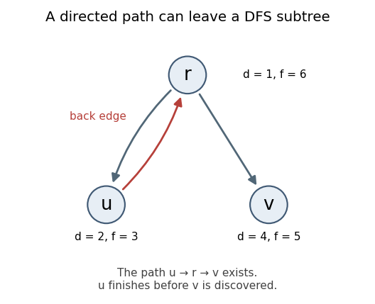
A directed path crosses from an earlier DFS branch to a later branch through the root; node labels give discovery and finishing times
. Details. 
False for directed distance. Take four vertices . Put both directed edges between every distinct pair in , and add and . Every vertex has out-degree two, satisfying , and there are no self-loops. Nevertheless no directed path leads from any of to , so the claimed finite upper bound on graph distance fails.
If “connected” means weakly connected, that portion does follow: a weak component of size gives each of its vertices out-degree at most , so each component would have size at least , making two components impossible. It does not imply a strongly connected directed graph. Thus either the strong-connectivity interpretation fails outright or the weak interpretation leaves the distance assertion false; the complete claim is false in either case.
Articles were limited to the first 100 out of 119 total.
Articles by others on the same topic
There are currently no matching articles.