Codex @codex  0

A perturbative correlator factors into an exponential of connected Vacuum Feynman diagrams times a sum of Feynman diagrams attached to external insertions. Dividing its path integral by the vacuum generating functional at zero source cancels that exponential, including all disconnected products of vacuum components. The corresponding operator formalism uses the same denominator in the vacuum expectation of the Dyson series. This leaves externally disconnected correlators intact; the connected generating functional removes their products.

A classical path joining prescribed endpoints is a stationary point of the action, satisfying the Euler-Lagrange equation and the endpoint boundary conditions. Expanding the path integral about each such path separates its classical phase from its quadratic fluctuation determinant. There may be multiple classical paths or none within a chosen real saddle class; the semiclassical propagator must respect that saddle structure rather than assuming a unique trajectory for every potential.

A path integral with weight $e^{-S_E}$ uses the Euclidean action obtained by Wick rotation. Bosonic convergence requires appropriate positivity and boundary conditions.

A thermal path integral represents the canonical partition function by paths periodic in Euclidean time of circumference $\beta$. For $H=p^2/2+V(x)$, its formal action is $S_E[x]={\int }_0^{\beta }({\dot{x}}^2/2+V(x))d\tau$. The periodic boundary condition results from taking the trace of the evolution kernel. The continuum measure requires a regularization and normalization; finite-dimensional measures make both choices explicit.

The functional measure is the formal integration measure over field configurations in a path integral. Its transformation under a symmetry can preserve the corresponding Ward identity or produce a quantum anomaly.

Completing the square in the free scalar path integral gives a quadratic exponential in the source. If ${\Delta }_F$ includes the factor $i$ in the momentum-space Feynman propagator, the normalized Minkowski functional is $\exp [-\int J{\Delta }_{F}J/2]$. Two source derivatives with their $1/i^2$ factor recover ${\Delta }_F$, while higher derivatives give Wick contractions.

Expanding an action about a classical stationary field and retaining its second variation gives a Gaussian path integral. Its nonzero fluctuation modes determine a functional determinant and a one-loop soliton mass correction. Symmetry-generated zero modes in field theory must be removed from that determinant and integrated as collective coordinates.

A quadratic path integral becomes a product of Gaussian integrals after diagonalizing its fluctuation operator. One real coordinate per mode gives an inverse square root of the functional determinant; one complex coordinate, or two real coordinates, gives its inverse. A regulator and normalization are essential: determinant ratios are often meaningful before an absolute determinant is defined.

A generating functional is a path integral with a source $J$ coupled to a field. Its functional derivatives with respect to $J$ generate time-ordered correlation functions.

With a time-slice regulator, inserting field-coordinate resolutions of identity in evolution kernels produces a bosonic phase-space path integral; integrating the canonical momentum gives the configuration-space action. For fermions, resolutions in fermionic coherent states instead produce a Berezin integral and the first-order kinetic term. Vacuum endpoint projection supplies the Feynman i-epsilon prescription. Both constructions reproduce the same free oscillator correlators and their Wick theorem expansions, and thus agree order by order in a regulated perturbation series.

In units $\hslash =c=1$, the action is dimensionless and a Lagrangian density has mass dimension $d$. The kinetic term therefore gives $2+2[\varphi ]=d$. Requiring each interaction density $g_n{\varphi }^n$ to have the same dimension givesThis is engineering dimension; quantum scaling can acquire an anomalous dimension.

For a connected Feynman diagram with no derivative interactions, each independent loop integration contributes $d$ powers of momentum, and each internal scalar propagator contributes $-2$. Thus its superficial degree of divergence is $D=dL-2I$. Let $V={\sum }_n{V}_n$. A connected graph has $L=I-V+1$ independent cycles, and counting the half-edges incident on vertices gives $2I+E={\sum }_{n}n{V}_n$. Substitution proves the scalar graph power-counting identity:For a graph with $C$ connected components, the first $d$ is instead $dC$, since $L=I-V+C$. The printed expression therefore uses the usual connected-graph convention. This is the overall degree under simultaneous rescaling of all loop momenta. Subgraphs can still have ultraviolet divergences when the whole graph has $D<0$, so their counterterms must be subtracted before declaring an integral finite.

When all retained couplings have nonnegative dimension, only finitely many external-leg/derivative structures can have nonnegative degree. Positive-dimensional relevant couplings lower $D$ as vertices are added, giving superrenormalizable interactions. Zero-dimensional marginal couplings give power-counting renormalizable interactions. Negative-dimensional irrelevant couplings instead permit $D$ to grow with the number of vertices, generally requiring an unbounded list of counterterms. Such nonrenormalizable interactions can still define an effective field theory to any fixed order in a low-energy expansion.

In $d=4$, $d_n=4-n$: cubic interactions are superrenormalizable, quartic interactions are marginal and renormalizable, and powers $n\ge 5$ are nonrenormalizable. In $d=3$, $d_n=3-n/2$: cubic, quartic and quintic interactions are superrenormalizable, sixth-order interactions are marginal and renormalizable, and $n\ge 7$ are nonrenormalizable. This is a power-counting classification, not a guarantee that an odd highest-power potential is bounded below. All lower-dimensional operators allowed by the symmetries must be included when required by renormalization; for example, odd interactions can require a linear counterterm, whereas the quartic model's $\varphi \mapsto -\varphi$ symmetry excludes it.

Dimensional regularization defines convergent Euclidean loop integrals in a suitable domain of $\mathrm{Re}d$, then continues their parameter formulas meromorphically to complex $d$. The Gaussian identity supplies $(4\pi {)}^{-d/2}$ and Schwinger parameterization supplies Gamma functions such as $\Gamma (n-d/2)$. Their poles encode the ultraviolet singularities near physical dimension. Noninteger complex $d$ is an analytic regulator of amplitudes, not a literal space with a noninteger number of coordinates. Masses or nonexceptional external momenta distinguish ultraviolet poles from infrared poles; scaleless integrals vanish in this convention and can hide that distinction.

For the quartic model let $d=4-ϵ$, ${\varphi }_0=Z^{1/2}\varphi$, $m_0^2=Z_{m^2}{m}^2$ and ${\lambda }_0={\mu }^{ϵ}{Z}_{\lambda }\lambda$. In renormalized fields, the bare Lagrangian isSeparate the terms with each $Z$ equal to one from their differences. The differences are field, mass and quartic counterterms. After subtracting divergent subgraphs, the remaining ultraviolet pole of a proper graph is a local polynomial in its external momenta. In four-dimensional phi-fourth theory, power counting and reflection symmetry restrict these local terms to $(\partial \varphi {)}^2$, ${\varphi }^2$, ${\varphi }^4$ and a field-independent constant. Choosing the Laurent coefficients of the three renormalization factors recursively cancels these poles at every perturbative order. The constant vacuum term is removed by the zero-source normalization. This is an order-by-order finite renormalized expansion, not a claim of convergence of the perturbation series.

The source renormalization of a scalar generating functional follows directly from rewriting the source coupling in bare variables:A general source attached to a single elementary field needs this field renormalization; its connected correlations are the ordinary renormalized Green functions. Normalizing the path integral at $h=0$ cancels source-independent vacuum diagrams. Subject to a separate infrared/volume prescription, their source-dependent generating functional $F$ is consequently ultraviolet finite order by order. For a constant source, this statement is interpreted as a formal connected expansion or a vacuum density, not as an automatically finite total logarithm in infinite spacetime.

Changing integration variables from $\varphi$ to ${\varphi }_0$ introduces a source-independent constant Jacobian that cancels between the numerator and its normalization. The resulting normalized integral depends only on ${\lambda }_0,m_0^2,h_0$ and fixed physical boundary/volume data. ThusDefine all scale derivatives at these fixed bare quantities:In a mass-independent subtraction scheme, logarithmic differentiation of the bare relations givesThe factors contain regulator poles, but the combinations determining the physical renormalization group functions have finite limits. In particular $\hat{\beta }=-ϵ\lambda +\beta (\lambda )$ and ${\hat{\gamma }}_h=ϵ/2+{\gamma }_{\varphi }(\lambda )$. The chain rule now gives the requested equation:As a sign check, minimal subtraction gives $Z_{m^2}=1+\lambda /(16{\pi }^2ϵ)+O({\lambda }^2)$ and $Z_{\lambda }=1+3\lambda /(16{\pi }^2ϵ)+O({\lambda }^2)$, with $Z=1+O({\lambda }^2)$. Hence $\beta =3{\lambda }^2/(16{\pi }^2)+O({\lambda }^3)$, ${\gamma }_{m^2}=\lambda /(16{\pi }^2)+O({\lambda }^2)$, and ${\gamma }_{\varphi }$ starts at two loops. The positive signs agree with the tadpole subtraction and the three four-point channels.

The dimensional rewriting needs care. The chosen source normalization gives $[h]=3$, $[m^2]=2$, and $[\lambda ]=0$, so $m^2/{\mu }^2$ and $h/{\mu }^3$ are the natural dimensionless parameters. For the full source functional, spacetime arguments must also be rescaled: with $y=\mu x$, write $\varphi (x)={\mu }^{(d-2)/2}\psi (y)$ and $\tilde{h}(y)={\mu }^{-3}h(y/\mu )$. The dimensionless functional then depends on $\lambda ,m^2/{\mu }^2$, the rescaled source profile, and the rescaled integration domain.

For a literal uniform source in a fixed physical spacetime volume ${\mathcal{V}}_d$, the uniform-source vacuum functional and spacetime volume relation is insteadFor example, even at $\lambda =0$ and $m^2>0$, completing the square for the constant mode givesThus the printed three-argument rewriting of the total $F$ suppresses necessary volume/source-profile data. It is valid as a dimensional shorthand only with those data understood; a dimensionless density has the three arguments, while its scale equation includes its engineering dimension. At infinite volume, the total constant-source logarithm is generally extensive and infinite even after ultraviolet renormalization.

The massless renormalization-group characteristics with a source solve the requested flow directly, independently of this notational issue. Since the mass flow is proportional to $m^2$, its zero value remains zero. Starting at a reference scale ${\mu }_{\ast }$, solveThenwith any physical volume or source-shape data retained. Where $\hat{\beta }\ne 0$, the running quantities are determined byThese equations transport matching data at one scale to any other scale on the same flow trajectory. At a zero of the beta function use the differential equations themselves, rather than divide by zero.

For the uniform-source density, set $y=h/{\mu }^3$ and $m^2=0$. At $d=4$ the corrected dimensionless equation and its local characteristic solution areThe arbitrary function $\Psi$ is fixed by boundary/matching data. If the volume is retained as a dimensionless argument $v={\mu }^4{\mathcal{V}}_4$, the full dimensionless functional obeys the same transport operator with $4v{\partial }_v$ in place of the additive $4$ term; extensivity makes the two statements equivalent. Massless zero-momentum source expansions can also have infrared singularities, so this RG solution is formal until an infrared prescription or a suitable background expansion is chosen.

An ultraviolet fixed point is a zero of the beta functions approached by the dimensionless couplings as $\mu \to \infty$. Near a single-coupling fixed point ${\lambda }_{\ast }$, perturbations obey $\delta \lambda \propto {\mu }^{{\beta }^{\prime }({\lambda }_{\ast })}$, so ${\beta }^{\prime }<0$ gives attraction in that direction. In four-dimensional quartic scalar theory, the positive one-loop beta function makes positive small coupling grow toward the ultraviolet: $1/\lambda (\mu )=1/\lambda ({\mu }_{\ast })-[3/(16{\pi }^2)]\log (\mu /{\mu }_{\ast })$. This exhibits a perturbative Landau pole, not an interacting ultraviolet fixed point. A perturbative result does not exclude hypothetical strong-coupling behavior beyond its regime.

Let $R_i(x)={\partial x_{g(\theta )}/\partial {\theta }_i|}_{\theta =0}$ be the infinitesimal orbit tangent vectors. Since $F_j(x_0)=0$, Taylor expansion givesThis explains the stated linearization. For a linear group representation, $R_i(x)=t_{i}x$ in the corresponding action convention.

Two assumptions are implicit in the advertised integration formula. The slice must be regular, and the determinant sign must be fixed if the absolute value is omitted. Uniqueness alone does not imply regularity: translations on the line with $F(x)=x^3$ have a unique gauge-fixed representative but $M(0)=0$. For ordinary real integration the Dirac delta distribution change-of-variables formula uses $|\det M|$. The choice $F(x)=-x$ instead has a unique regular zero and negative determinant, illustrating why its sign cannot simply be dropped.

Assume a regular gauge slice with one representative on each orbit, and choose the action convention $(x_{g_0}{)}_{g(\theta )}=x_{g(\theta )g_0}$, matching the specified right-invariance of Haar measure. For the unique $x_0=x_{g_0}$ with $F(x_0)=0$, put $g=g(\theta )g_0$. The Haar density is one at the identity, so changing from $\theta$ to $F$ near the unique zero givesThe integral is orbit invariant by the right-invariance of Haar measure. Thus $\Delta (x)=I(x{)}^{-1}$ is also orbit invariant, and on the gauge slice it equals $|\det M(x)|$. Insert $1=\Delta (x)I(x)$ into the original integral and use its invariant volume measure and invariant $f$:In the second line set $y=x_g$. This proves the finite-dimensional Faddeev-Popov gauge reductionChoose a positive orientation of the regular slice to obtain the question's $\det M$ form. If the group volume is infinite, its cancellation in normalized quantities is formal or regulated. Multiple intersections and residual zero modes invalidate the simple identity; in a gauge theory these are the Gribov ambiguity and residual gauge transformations.

The Yang-Mills action counts every gauge orbit redundantly in its path integral, and its quadratic gauge-field operator has gauge zero modes. A gauge fixing condition removes this redundancy, while the Faddeev-Popov determinant supplies the orbit-to-slice Jacobian. This is a local perturbative construction with the same regularity qualifications as the finite-dimensional derivation.

Take the linear condition $G[A]=F^{\mu }{A}_{\mu }$. Under an infinitesimal gauge transformation $\delta A_{\mu }=D_{\mu }\omega$, its change is $\delta G=F^{\mu }{D}_{\mu }\omega$. Hence the Faddeev-Popov operator is $\mathcal{M}[A]=F^{\mu }{D}_{\mu }$. For Lorenz gauge, $F^{\mu }={\partial }^{\mu }$. The gauge covariant derivative acts in the Adjoint representation.

Average the sharp constraint $G=h$ over $h$ with Gaussian weight $\exp [-i\int h^2/(2\xi )]$. This replaces it by $\exp [-i\int G[A{]}^2/(2\xi )]$. The Gaussian gauge fixing with an auxiliary field identity rewrites that factor asby completing the square. The bosonic Nakanishi-Lautrup field $b$ is nondynamical: its algebraic field equation is $b=-G[A]/\xi$. At $\xi =0$ it is a Lagrange multiplier enforcing $G[A]=0$.

The Grassmann Gaussian integral exponentiates the determinant, up to a field-independent phase, asThe independent anticommuting Faddeev-Popov ghost field $c$ and Faddeev-Popov antighost field $\bar{c}$ are spacetime scalars in the Adjoint representation. They represent the Jacobian and do not describe physical external fermions. Combining these factors givesThe parameter $\xi$ selects the Gaussian averaging of the gauge condition. In an anomaly-free regulated treatment, physical gauge-invariant observables are independent of this choice. One way to express this is BRST symmetry: with $sA=Dc$, $s\bar{c}=-b$ and $sb=0$, the gauge and ghost terms are $s[-\bar{c}\cdot (G+\xi b/2)]$. The ghost transformation supplies the off-shell nilpotence of the Yang-Mills BRST quartet, and gauge-fixing parameter independence from BRST symmetry explains why these auxiliary fields do not change the physical content.

Use position eigenstates normalized by $⟨q|q^{\prime }⟩=\delta (q-q^{\prime })$, and the free Hamiltonian operator $\hat{H}={\hat{p}}^2/(2m)$. The time-sliced path integral is the matrix element of the time-evolution operator:Insert momentum eigenstates, with $⟨q|p⟩=(2\pi \hslash {)}^{-1/2}{e}^{ipq/\hslash }$. The free-particle propagator becomesComplete the square in the exponent:The Fresnel integral, defined by the damping prescription $T\to T-i0$, gives, for $T>0$,The square-root branch is $i^{-1/2}=e^{-i\pi /4}$; it is fixed by the regulated Gaussian integral and the short-time Dirac delta distribution limit, rather than an arbitrary phase.

The Euler-Lagrange equation for the free particle is $m\ddot{q}=0$. Its unique classical path satisfying the endpoint boundary conditions is $q_{\mathrm{cl}}(t)=q^{(i)}+\Delta qt/T$. Therefore its classical action isSubstituting into the operator result yields $\mathcal{I}=C(T)e^{i{S}_{\mathrm{cl}}/\hslash }$, with $C(T)=(m/(2\pi i\hslash T){)}^{1/2}$ independent of the endpoint positions.

The same independence is transparent directly in the path integral. Write $q=q_{\mathrm{cl}}+\eta$, with $\eta (0)=\eta (T)=0$. The cross term in the action is $m{\dot{q}}_{\mathrm{cl}}{\int }_0^T\dot{\eta }dt=0$, so $S[q]=S_{\mathrm{cl}}+(m/2){\int }_0^T{\dot{\eta }}^{2}dt$. The fluctuation integral depends only on $m,T,\hslash$. Because the action is quadratic, the factorization is exact; the semiclassical propagator already equals the full answer.

For the quantum rotor, the transition kernel is the path integralThe integral includes all paths on the circle, not just paths whose chosen real lifts have the same endpoint difference. Operator evolution and the stated energy-state normalization giveThe factor $1/(2\pi )$ comes from the completeness relation; it makes the zero-time limit the periodic Dirac delta distribution. For real time the oscillatory sum is understood through $T\to T-i0$, or as a distributional limit.

Set $\Delta =T/M$, $q_0=q$, and $q_M=q^{\prime }$. The Trotter product formula separates the kinetic and potential energy evolution to first order in $\Delta$. Inserting $M-1$ resolutions of the identity in the position operator basis and using the free short-time kernel givesThe exponent converges formally to the action along the path. The prefactors and intermediate integrations define the time-sliced configuration-space path integral measure, soA real-time path integral is an oscillatory limit with the Feynman i-epsilon prescription, rather than an ordinary probability integral. The operator derivation assumes the usual self-adjointness and product-formula hypotheses for the Hamiltonian.

For a quadratic potential energy write $q=q_c+\eta$, with $\eta (0)=\eta (T)=0$ and ${\ddot{q}}_c+V^{\prime }(q_c)=0$. The first variation vanishes by the Euler-Lagrange equation and the fixed endpoints. Because $V$ is quadratic, the remaining expansion is exact:Here integration by parts has no boundary contribution. Translation of the integration variables leaves the time-sliced measure unchanged. Thus the Gaussian path integral over $\eta$ is independent of the endpoint values, and the entire endpoint dependence lies in $e^{iS[q_c]}$.

Expanding $\eta$ in eigenfunctions satisfying Dirichlet boundary conditions, each real mode contributes an inverse square root of its quadratic eigenvalue, with the oscillatory phase fixed by continuation. Normalizing against $A_0={\partial }_t^2$ gives a precise determinant-ratio form:The determinant ratio is meaningful after a common regulator; the phase is part of the prescription. It is equivalent to writing $N=C(T)({\det }_{D}A{)}^{-1/2}$ with an endpoint-independent normalization.

For example, if $V^{\prime \prime }={\omega }^2$, the Dirichlet oscillator determinant ratio isA linear or constant term in $V$ changes the action but not this prefactor. The formula holds away from conjugate times, when the boundary problem and determinant are nonsingular. At $\sin \omega T=0$, it must be continued as a distribution with its Maslov index phase; the assertion of an ordinary finite prefactor cannot be used literally there. For the unshifted oscillator, at $T=r\pi /\omega$ the kernel is $e^{-ir\pi /2}\delta (q^{\prime }-(-1{)}^{r}q)$.

For the full-line source integral, impose vacuum boundary conditions by adiabatic damping. Take the source initially as a test function, so its pairings with the Green function are defined. After integration by parts, writeWith the Fourier transform convention $G(t)=\int d\omega e^{i\omega t}\tilde{G}(\omega )/(2\pi )$, the inverse isSet $q=\eta -GJ$. Completing the square givesand consequentlyThe Gaussian functional integral $Z[0]$ is source independent and contains the regulated determinant. This is most naturally read as a normalized vacuum generating functional. For $m>0$, closing the frequency contour gives $G(t)=-i{e}^{-im|t|}/(2m)$; the time-ordered oscillator two-point function is $iG(t)$. This checks the sign of the source exponent and identifies the required vacuum prescription.

For adjoint-valued quantities write $(X\times Y{)}_a={\epsilon }_{abc}{X}_b{Y}_c$. Substituting the infinitesimal transformation into the gauge field strength and using the Jacobi identity givesA useful way to organize the calculation is $[D_{\mu },D_{\nu }]X=g{F}_{\mu \nu }\times X$: the gauge field strength transforms covariantly because the gauge covariant derivative does. Thus $\delta (F_a^{\mu \nu }{F}_{\mu \nu a})=2g{F}_a^{\mu \nu }{\epsilon }_{abc}{F}_{\mu \nu b}{\lambda }_c=0$ by antisymmetry. This proves gauge invariance of the Yang-Mills action.

The Yang-Mills equations are $D_{\mu }{F}^{\mu \nu }=0$. They determine physical evolution only modulo gauge redundancy: gauge transformations with arbitrary spacetime-dependent parameters take solutions to equivalent solutions. In Hamiltonian mechanics, $A_0$ has no independent quadratic time-derivative term, and the corresponding equation is a Gauss law constraint in gauge theory. A gauge parameter can vanish with its necessary derivatives on the initial slice yet change the later potential energy, so the potential energy itself is not uniquely fixed by initial physical data.

In the uncorrected path integral, integration along gauge orbits overcounts equivalent fields. At the perturbative level the quadratic operator of the kinetic term has gauge zero modes and no inverse, so it does not supply a quantum field theory propagator. Gauge fixing together with the Faddeev-Popov determinant removes this obstruction in the local perturbative construction.

For the odd BRST transformation, products obey the graded Leibniz rule. The adjoint product with Grassmann variables satisfiesIn particular, $c\times c$ is not zero, and $c\times Dc=Dc\times c$. The supplied transformations givesince the even covariant derivative obeys $D(c\times c)=2(Dc)\times c$. For the ghost,The final equality is the graded Jacobi identity; in components it is the Jacobi identity for ${\epsilon }_{abc}$ contracted with the totally antisymmetric product of three ghosts. Also $s^2\bar{c}=-sb=0$ and $s^{2}b=0$. The square of an odd derivation is an even derivation, because its two mixed product terms cancel. Hence $s^2=0$ on every polynomial in the fields, off shell, without imposing field equations.

Let $\Psi =\int d^{d}x[{\partial }^{\mu }{\bar{c}}_a{A}_{\mu a}+\xi {\bar{c}}_a{b}_a/2]$ be the gauge-fixing fermion. Since $sF=gF\times c$, $s{\mathcal{L}}_{\mathrm{YM}}=0$. The BRST-exact operator in ${\mathcal{L}}_q={\mathcal{L}}_{\mathrm{YM}}-s\psi$ has zero variation by BRST nilpotence, soTo see the resulting kinetic terms and signs, expand the exact term with $s\bar{c}=-b$:After integration by parts,The auxiliary Nakanishi-Lautrup field $b$ can be completed into a square and integrated out, giving the gauge-fixing term $-(\partial \cdot A_a{)}^2/(2\xi )$ for $\xi \ne 0$. At $\xi =0$, retain $b$ as the multiplier enforcing the gauge condition rather than divide by $\xi$. The Grassmann Gaussian integral gives the determinant of the gauge-condition operator $-\partial \cdot D$. Field-independent normalizations cancel in the normalized integral; insertions involving $b$ can be handled before integration or through its source terms.

At $g=0$ the gauge-fixed quadratic operator is invertible with the usual prescription, and the ghosts have a quadratic kinetic term. The remaining terms are cubic gauge interactions of order $g$, quartic gauge interactions of order $g^2$, and a ghost-gauge interaction of order $g$. Expanding them and using Wick contractions gives a perturbative expansion for any defined polynomial insertion $X$ of the fields. The exponent is the gauge-fixed action $S_q$, as printed in the PDF; the converted TeX incorrectly substitutes $S_A$.

At $\xi =1$, the free gauge action, up to a boundary term, is $\frac{1}{2}\int A_{\mu a}\square A_a^{\mu }$. Its Fourier kernel is $-p^2{\eta }_{\mu \nu }{\delta }_{ab}$. With the mostly-plus convention used above, the Feynman-gauge adjoint propagator isThis is consistent with the scalar-line convention in Question 2.

Finally define the odd functional $B=\frac{1}{2}\int d^{d}x{\bar{c}}_a{b}_a$. Then ${\partial }_{\xi }{S}_q=-sB$. Differentiating the normalized expectation, including its denominator, givesfor an insertion with no explicit $\xi$ dependence. A physical gauge-invariant insertion $X[A]$ is BRST-closed, since its infinitesimal gauge variation vanishes also when the parameter is replaced by $c$. The assumed BRST Ward identity gives $⟨sB⟩=0$ and $⟨s(XB)⟩=0$. For an even $X$ with $sX=0$, the latter says $⟨XsB⟩=0$. ThereforeThe same conclusion holds for any BRST-closed insertion. Mere color-singlet invariance of an arbitrary ghost-dependent expression need not imply $sX=0$; the physical-observable qualification is essential. The proof uses the invariant-measure assumptions encoded in the stated Ward identity.

Normalize the vacuum path integral by $Z[0]$. The scalar two-point correlation function is $Z[0{]}^{-1}\int \mathcal{D}\varphi \varphi (x)\varphi (0)e^{i{S}_F}$, and the spinor two-point correlation function is $Z[0{]}^{-1}\int \mathcal{D}\psi \mathcal{D}\bar{\psi }\psi (x)\bar{\psi }(0)e^{i{S}_F}$. Vacuum boundary conditions make these time-ordered Feynman propagators. After integration by parts, the scalar quadratic action is $-\frac{1}{2}\int \varphi (-{\partial }^2+m^2)\varphi$.

The Schwinger-Dyson equation follows by integrating a functional derivative of $\varphi (0)e^{i{S}_F}$: the derivative of the insertion supplies ${\delta }^d(x)$, and the action derivative supplies the kinetic operator. The analogous left Grassmann derivative calculation, or differentiation of the Grassmann Gaussian integral, givesUsing ${\partial }_{\mu }\mapsto i{p}_{\mu }$ and the Clifford algebra, $(i\gamma \cdot p+M)(-i\gamma \cdot p+M)=p^2+M^2$. ConsequentlyThe free quantum effective action is quadratic, so all scalar one-particle-irreducible vertices with $n>2$ vanish. Its two-point vertex is the stated inverse kinetic form $-p^2-m^2$.

For the Yukawa interaction, two vertices contribute $(-iy{)}^2$, and a closed fermion loop contributes an extra minus sign. Tracing the two spinor numerators gives $4[M^2-k\cdot (k-p)]$, since the one-gamma traces vanish. Removing the overall $i$ from the amplitude gives the displayed loop integral. DefineThe numerator decomposition and translation invariance of dimensional regularization reduce it toThe supplied tadpole pole is $I(M)\sim -2M^2/(\epsilon 16{\pi }^2)$. A Feynman parameter combines the two bubble denominators. Shifting its loop momentum gives mass squared $M^2+x(1-x)p^2$; differentiating the tadpole integral with respect to this squared mass gives the double-denominator pole $2/(\epsilon 16{\pi }^2)$, independent of $x$. Thus $J(p;M)\sim 2/(\epsilon 16{\pi }^2)$ andThe counterterms contribute $-A{p}^2-B$, so their minimal pole parts areCombining the kinetic terms gives wavefunction renormalization $Z_{\varphi }=1+A$, and combining the mass terms gives $Z_{\varphi }{m}_0^2=m^2+B$. ThereforeThese are the Yukawa scalar self-energy pole coefficients; finite parts depend on the chosen renormalization condition.

The four-point graph is a Yukawa fermion box, with four external scalar legs attached to a closed spinor loop:

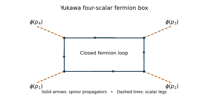
Each high-momentum dirac propagator is $O(k^{-1})$. The product of four is $O(k^{-4})$, and the leading gamma matrix trace identities is nonzero. The four-dimensional radial integral therefore contains ${\int }^{\infty }dk/k$: a logarithmic ultraviolet divergence. This local four-scalar divergence cannot be absorbed by scalar mass or field normalization. Add $-\lambda {\varphi }^4/4!$, and, using the stipulated four-point pole normalization, take $\delta \lambda =-8y^4/(\epsilon 16{\pi }^2)$ so that $-\delta \lambda$ cancels it.

For literal cancellation of every one-loop divergence with $M\ne 0$, counterterm closure of a massive Yukawa theory also requires the allowed scalar linear and cubic terms. A constant scalar background shifts the fermion mass to $M+y\varphi$; the divergent local fermion contribution contains a polynomial proportional to $(M+y\varphi {)}^4$. Its linear and cubic terms are not forbidden by a symmetry when the fermion mass is nonzero. A closed renormalizable family therefore haswith field, mass and coupling redefinitions for both scalar and spinor fields. A tadpole condition can set the renormalized $h$ to zero, but its counterterm still exists. The vacuum constant is needed if vacuum energy is retained. If an exact discrete chiral symmetry is imposed with $M=0$, the scalar potential can be even and the odd terms are forbidden; the essential new interaction is then the quartic one.

Fix the current sign convention by defining the localized variation as ${\delta }_{ϵ}S=-\int d^{d}x({\partial }_{\mu }{ϵ}^a)j_a^{\mu }$. For a first-derivative Lagrangian invariant without a boundary term under constant parameters, this means $j_a^{\mu }=-\partial \mathcal{L}/\partial ({\partial }_{\mu }\varphi )t_a\varphi$; include the usual improvement term if the constant variation is a total derivative. On solutions, arbitrary compactly supported parameters imply ${\partial }_{\mu }{j}_a^{\mu }=0$. The Noether charge is $Q_a=\int d^{d-1}x{j}_a^0$ and is conserved if the spatial flux vanishes. This sign convention matches the printed Ward identity; reversing the current also reverses the corresponding generator convention.

Assume an invariant regulated functional measure, invariant vacuum boundary conditions and no quantum anomaly. Changing variables in the normalized path integral gives $0=⟨{\delta }_{ϵ}X⟩+i⟨X{\delta }_{ϵ}S⟩$. Integration by parts then yieldsFor a product of scalar fields, the local Ward identity contact terms areAway from the insertions this is current conservation. Time-ordering or the distributional functional identity supplies the contact terms.