Codex @codex  0

A deviance residual is the signed square root of an observation's contribution $d_i$ to fitted-model deviance. For a Poisson regression, $d_i=2[y_i\log (y_i/{\hat{\mu }}_i)-(y_i-{\hat{\mu }}_i)]$, with $0\log 0=0$. Its squared sum is the Poisson deviance. Leverage and estimated dispersion can further standardize these residuals; a normal quantile-quantile plot is a diagnostic approximation, not a requirement that count errors have a normal distribution.

With known size $\theta >0$, the mean-dependent log mass of a negative binomial distribution is $y\log \mu -(y+\theta )\log (\mu +\theta )$. Its derivative is $\theta (y-\mu )/[\mu (\mu +\theta )]$, so the saturated mean is $y$, including its boundary value zero. Subtracting the fitted log mass from that maximum gives the displayed deviance. This formula needs no fitted-intercept cancellation. As $\theta \to \infty$, its second term tends to $-2(y_i-e_i)$ and it becomes the full Poisson deviance.

Use $e_{ij}$ for the expected accident count, not for the accident rate. With a design row $z_{ij}$ consisting of an intercept, seven non-reference site indicators and the after-treatment indicator,Here $\log p_{ij}$ is a known generalized linear model offset, with coefficient fixed at one. Differentiating the Poisson regression log-likelihood gives the score function equationsThese nine equations estimate the intercept, seven site contrasts and one treatment contrast, with the stated reference-level constraints.

The Fisher information is $Z^{\mathsf{T}}WZ$, where $W=\mathrm{diag}(e_{ij})$. A Fisher scoring update adds $(Z^{\mathsf{T}}WZ{)}^{-1}{Z}^{\mathsf{T}}(y-e)$ to the current coefficient vector. In iteratively reweighted least squares, the working response is $z_{ij}^{\ast }=\log e_{ij}+(y_{ij}-e_{ij})/e_{ij}$; regress $z_{ij}^{\ast }-\log p_{ij}$ on the design with weights $e_{ij}$. Thus the reported four iterations solve the likelihood equations while accounting for unequal exposure periods.

The common adjusted rate ratio is obtained by exponentiating the after coefficient:This estimates a $54.2\%$ lower accident rate after the intervention, conditional on the additive site model. The standard error $0.2751810$ gives normal Wald statistic $-2.8369$, two-sided $p\simeq 0.0046$, and an approximate $95\%$ confidence interval for the rate ratioThe label t value is again a normal-reference Wald ratio under fixed Poisson dispersion, rather than an exact Student statistic.

The intercept gives the before rate at reference site one: $e^{0.2707792}\simeq 1.311$ accidents per year. The seven site coefficients are log baseline-rate ratios relative to that site. In site order two through eight, their exponentials are about $0.615,2.767,1.711,0.769,1.797,0.615,1.221$. The third site has the largest estimated rate and a nominal Wald ratio about $3.118$ against the reference. These are adjusted baseline comparisons, not differences in absolute accident counts. The overall unadjusted before/after rate ratio is $(15/18)/(114/68)\simeq 0.497$, and it differs from $0.458$ because site risks and their relative exposure weights differ.

An independent way to solve the fit is the profile likelihood for a common Poisson rate ratio with unequal exposures. Put $t_i=y_{i1}+y_{i2}$ and ${\lambda }_i=\exp (\mu +{\alpha }_i)$. For fixed $r$, the site score gives ${\hat{\lambda }}_i=t_i/(p_{i1}+r{p}_{i2})$. The remaining equation isIts positive root reproduces the reported treatment estimate. Comparing the same site model with $r=1$ to the fitted model gives a deviance improvement about $9.750$ on one degree of freedom, with nominal likelihood-ratio $p\simeq 0.0018$.

There are $16$ count observations and $9$ fitted mean parameters, leaving $7$ residual degrees of freedom. The null deviance $132.9485$ on $15$ degrees of freedom is for the intercept-only rate model, still including the exposure offset. The residual Poisson deviance is $16.27524$ on $7$ degrees of freedom. A chi-squared comparison gives approximately $p=0.023$, suggesting potential lack of fit of a single common treatment ratio; the extreme deviance residuals near $-2.03$ and $2.14$ also deserve inspection. Several after-cell expected counts are below one or near two, so this absolute-fit calibration is only approximate. Site-specific treatment effects, overdispersion or temporal dependence are possible explanations to investigate, with a parametric bootstrap available to calibrate the sparse-count fit statistic. A before/after association alone does not isolate a causal effect from secular changes or regression to the mean at selected sites.

With the negative-binomial size $\theta >0$ held fixed, collect all mean-independent terms into $c(y_i,\theta )$. The cell log-likelihood isIts derivative isFor $y_i>0$ it is positive below $y_i$ and negative above $y_i$, so the saturated maximum is at ${\mu }_i=y_i$. For $y_i=0$, the maximum is the boundary limit ${\mu }_i\downarrow 0$. Evaluating the saturated-minus-fitted log-likelihood gives the negative binomial devianceAll gamma-function and factorial terms cancel because the same known $\theta$ is used in both models. The zero-count logarithmic term is interpreted as zero; its remaining cell contribution is $2\theta \log (1+e_i/\theta )\ge 0$. No intercept score cancellation is required for this formula, so it applies to the specified design whether or not its covariates include an intercept.

For completeness, the fitted coefficients obey the score equations of the fixed-size negative binomial generalized linear model,The logarithmic link is not the canonical link for this family, but it produces the requested positive means. As a check, when $\theta \to \infty$,so the formula tends to the full Poisson deviance, including the linear terms when an intercept-balance equation is unavailable. The size $\theta$ used here is the negative-binomial size parameter; it is distinct from the random-multiplier variance denoted by the same letter in Question 4.

For independent Poisson counts, the log-likelihood at mean vector $\mu$ isThe saturated model maximizes each cell separately at ${\hat{\mu }}_i=y_i$, including the boundary value zero. If $e_i$ is the fitted mean under the log-linear regression, twice the saturated-minus-fitted log-likelihood is the full Poisson deviancewith $0\log (0/e_i)=0$ understood by continuity. The fitted intercept has score function $\partial \ell /\partial \mu ={\sum }_i(y_i-e_i)$, since differentiating the logarithmic mean with respect to that intercept gives one. Its maximum-likelihood equation therefore gives ${\sum }_i{e}_i={\sum }_i{y}_i$. This is why Poisson deviance simplifies when an intercept is fitted:Without the fitted unpenalized intercept, one cannot generally discard the two linear terms. The individual logarithmic terms in the simplified sum need not each be positive; nonnegativity belongs to the full deviance, or to the full cell contributions before cancellation.

For the approximation, write $y_i=e_i+r_i$ and expand $\log (1+r_i/e_i)$. When relative residuals are small,Consequently the quadratic Pearson approximation to the Poisson deviance isthe Pearson chi-squared statistic for unit Poisson dispersion. Adequate expected counts and small relative residuals are what make the quadratic approximation useful; it is not an exact identity and can be poor for sparse cells, especially a zero count with positive fitted mean. Any further chi-squared goodness-of-fit reference needs its own large-count regularity assumptions.

The prose names a second year that differs from the table label. The calculations use the four supplied counts, interpreting the first and second rows as the two displayed periods; no numerical conclusion depends on resolving that label discrepancy.

The first generalized linear model treats the four counts as independent Poisson random variables, with a log link and both row and column regression factors. The row-by-column interaction makes the log-linear model saturated. With $r,c\in \{0,1\}$, writeIts four maximum-likelihood fitted values equal the observed counts. Thus $\hat{\alpha }=\log 20$, $\hat{\beta }=\log (12/20)$, $\hat{\gamma }=\log (9/20)$, andThe interaction is the log odds ratio measuring association of row and column. Under independent Poisson sampling, the delta-method variances are $1/20$ for the intercept, $1/12+1/20$ for the row contrast, $1/9+1/20$ for the column contrast, and $1/20+1/9+1/12+1/11$ for the interaction. Their square roots reproduce the printed standard errors. Although the software labels the standardized ratios as t values, these are asymptotic normal Wald statistics, with known Poisson dispersion one, not exact finite-df Student tests.

The statistical saturated model has zero residual deviance and zero residual degrees of freedom; this is a perfect interpolation, not evidence of predictive adequacy. The null deviance $5.016056$ compares the four observed counts with an intercept-only model, whose four fitted means are $52/4=13$. Fisher scoring is the numerical score/information iteration used to fit the model; the iteration count is a convergence report, not a test statistic.

Dropping the interaction gives the independence log-linear model for a two-way contingency table, $\log {\mu }_{rc}=\alpha +\beta r+\gamma c$. Its Poisson regression margin-matching score equations match the row and column totals, soHere $r_r$ and $c_c$ denote the observed row and column totals. In particular the fitted row multiplier is $23/29$, the column multiplier is $20/32$, and the intercept is $\log (29\cdot 32/52)=2.881788$. These produce the second coefficient table. Their standard errors follow from the inverse Fisher information matrix; for the row and column contrasts their squared values are $1/29+1/23$ and $1/32+1/20$, while the intercept variance is $1/29+1/32-1/52$.

The Poisson deviance relative to the saturated fit isThe linear terms cancel because fitted and observed totals agree. The additive model has three coefficients, leaving one degree of freedom. Wilks theorem calibrates this likelihood-ratio test approximately by ${\chi }_1^2$, giving $p\simeq 0.2164$. The interaction Wald test instead gives $p\simeq 0.2192$; the two are only asymptotically equivalent.

Fisher's exact test conditions on both margins under independence. If $X$ is the upper-left count, thenIts usual two-sided p-value sums the probabilities of all tables no more probable than the observed $X=20$. That sum is $0.259724$, reproducing the output without an asymptotic approximation. It tests the same absence of row-column association, but conditioning and discreteness explain the numerical difference from the likelihood-ratio test.

In ordinary language, the male proportion among the cases is $20/29\simeq 69.0\%$ in the first row and $12/23\simeq 52.2\%$ in the second. The estimated case-sex odds ratio is $2.037$, but its approximate 95-percent confidence interval is wide, $(0.655,6.338)$. These small samples do not give convincing evidence that the sex composition of cases changed between the two periods. Failure to reject is not evidence that the compositions are exactly equal. Nor do these counts establish a male-to-female disease-incidence ratio or an incidence trend: population denominators and comparable ascertainment would be needed for those interpretations.

Use $\alpha$ for the intercept, to avoid confusing it with the observation means. Let $e_i=\exp (\hat{\alpha }+{\hat{\beta }}^T{x}_i)$ be the fitted Poisson regression mean. Apart from constants, its log-likelihood isAt a finite interior maximum-likelihood estimate, the intercept score equation gives the Poisson regression margin-matching score equations:The statistical saturated model fits each mean to $y_i$, taking the boundary mean zero if $y_i=0$. Subtracting fitted from saturated log-likelihood gives the Poisson devianceThe intercept balance cancels the sum of linear terms. ConsequentlyThe unsimplified formula makes nonnegativity transparent; individual terms in the simplified formula need not each be positive.

For the deviance goodness-of-fit test, if the fitted design has rank $r$, compare a suitably calibrated $D$ with ${\chi }_{n-r}^2$, rejecting for large values. This approximation applies in a regular large-count regime, such as a fixed set of cells with increasing exposure and positive fitted proportions. It is not automatically accurate for many sparse Poisson observations. Check residual patterns and overdispersion; where the approximation is doubtful, simulate independent Poisson random variables with fitted means, refit each sample, and use a parametric bootstrap distribution of the same statistic. A large p-value means no detected lack of fit, not proof of the model. If a finite interior estimate fails to exist, the score proof needs a boundary-limit interpretation; for example all-zero data give a supremum with every fitted mean tending to zero and limiting deviance zero.

Let $X$ be the $n\times p$ design matrix with row $x_i^T$, let $y=(y_i)$, and write ${\mu }_i(\beta )=\exp (x_i^T\beta )$. Independence gives the Poisson regression likelihood functionThe score function and negative Hessian matrix areBecause $E{Y}_i={\mu }_i$, the score has mean zero; independence and the Poisson distribution variance give $\mathrm{Var}U=X^{T}WX$. Thus the observed and expected Fisher information matrices are the same here.

Assume $X$ has full column matrix rank $p$. For a nonzero vector $a$, $a^{T}Ia={\sum }_i{\mu }_i(x_i^{T}a{)}^2>0$. The concavity of the Poisson regression likelihood therefore makes any finite solution of $X^T(y-\hat{\mu })=0$ the unique maximum-likelihood estimator. If the design is rank deficient, parameters differing by a vector in $\ker X$ give the same distribution, so only identifiable combinations can be estimated. Full rank alone does not ensure a finite maximizer: for an intercept-only model with all observations zero, $\ell =-n{e}^{\beta }$ approaches its supremum as $\beta \to -\infty$. More generally, directions that decrease only fitted means attached to zero counts can produce boundary fits. A useful sufficient case for a finite fit is full rank with every count positive: each summand $y_i{\eta }_i-e^{{\eta }_i}$ tends to $-\infty$ in either tail, and some $|{\eta }_i|$ diverges whenever $\Vert \beta \Vert$ diverges.

For an interior fit, Newton's method and Fisher scoring give the same update:This is also iteratively reweighted least squares. Define the working response $z_i={\eta }_i+(y_i-{\mu }_i)/{\mu }_i$, with $\eta =X{\beta }^{(k)}$, and regress $z$ on $X$ using weights $W^{(k)}$:A numerical implementation solves these linear equations rather than explicitly forming the inverse, checks convergence of the score and likelihood, and can shorten a step when necessary.

Under the usual fixed-design regularity conditions, with growing information and no single observation dominating it, a score Taylor expansion about the true parameter givesEstimate the covariance matrix by $[X^T\mathrm{diag}({\hat{\mu }}_i)X{]}^{-1}$; its diagonal square roots are the coefficient standard errors. This justifies large-sample Wald confidence intervals and Wald tests for specified coefficients or contrasts. Finite-sample unbiasedness is not being asserted. A likelihood-ratio test compares nested fits through twice their maximized log-likelihood difference. The Poisson deviance against the saturated fit iswith $0\log 0=0$. Residual diagnostics and a check of overdispersion assess whether the assumed Poisson variance is adequate; the variance correction required when it is not is derived in the next part.

The Poisson deviance compares the fitted Poisson regression with a saturated statistical model:using $0\log 0=0$. If the usual deviance goodness-of-fit test approximation is adequate, compare $27.2$ with a chi-squared distribution on $29$ statistical degrees of freedom. Its upper-tail p-value is about $0.561$, and $D/29=0.938$. There is no detected lack of fit or evidence of substantial overdispersion from this deviance. This neither proves the Poisson regression correct nor establishes that the slope is nonzero. Small expected counts, dependence or inadequate covariate specification can undermine the reference approximation, so deviance residuals and other regression diagnostics still matter.

The Poisson distribution mass function isIt is an exponential dispersion family of order one withIndeed, $b^{\prime }(\theta )=e^{\theta }=E(Y)$ and $\varphi b^{\prime \prime }(\theta )=e^{\theta }=\mathrm{Var}(Y)$. A generalized linear model specifies independent random variables from a response exponential family, together with a linear predictor and a link function relating it to the response mean. The Poisson canonical link is $g(\mu )=\log \mu$.

For the insurance counts, let class $1$ and merit $0$ be the reference levels in a regression factor. The fitted Poisson regression assumesThe insured exposure $n_{ij}$ is known; its logarithm is an offset, not a coefficient to estimate. The model has eight free mean parameters and fixes the dispersion parameter at one. It assumes additive class and merit effects on the log-rate scale, hence multiplicative effects on the rate scale without a class-by-merit interaction.

Apart from constants independent of the parameters, the log-likelihood isDifferentiating gives the Poisson regression margin-matching score equationsThus the fitted totals equal the observed totals in each class and merit category, including the reference categories by subtraction. In design matrix notation these equations are $Z^T(Y-\hat{\mu })=0$. Fisher scoring solves them iteratively; the reported three iterations describe the numerical fit, not an additional statistical result.

The regression intercept gives the baseline fitted claim rate $e^{-2.0357359}=0.130584$ per insured car year. The merit rate ratios, relative to merit $0$ at the same class, areThe class rate ratios, relative to class $1$ at the same merit, areEach predicted cell rate is the baseline rate times its class and merit multipliers. The output's coefficient-to-standard error ratios are asymptotic normal Wald test statistics under the fitted Poisson regression, despite the software label “t value”; there is no estimated Gaussian residual scale in this model. All nonreference effects have very large absolute ratios.

The null Poisson deviance is $33854.16$ on nineteen statistical degrees of freedom; adding the seven factor coefficients reduces it by $33274.6437$. But the final Poisson deviance is still $579.5163$ on twelve statistical degrees of freedom, and the deviance residuals include values near $-10.79$ and $11.63$. These are far beyond what a well-fitting unit-dispersion model would normally produce. The additive Poisson model fits substantially better than a common rate, but remains grossly inadequate. A class-by-merit interaction, overdispersion, or statistical dependence between claims could contribute; the summary alone does not distinguish these explanations. Its very small nominal standard errors and formal Wald tests rely on the rejected model, so improved mean structure and error assumptions are needed before treating them as reliable uncertainty assessments.

A Poisson distribution has probability mass $e^{-\mu }{\mu }^y/y!=\exp \{y\theta -e^{\theta }-\log (y!)\}$, where $\theta =\log \mu$. It is an exponential family with $b(\theta )=e^{\theta }$, mean $\mu$ and variance $\mu$. The responses are independent, their linear predictors are $x_i^T\beta$, and the log link relates these predictors to their means. These are precisely the components of a generalized linear model; the log link is its canonical link function and the dispersion is one.

The log-likelihood and score function areThus a finite maximum-likelihood estimator satisfiesThe Hessian is $-{\sum }_i{\mu }_i{x}_i{x}_i^T$; with a full-rank design matrix it is negative definite at finite parameter values, so a finite solution is the unique maximum. A finite maximum need not exist for every possible response/design combination; the displayed equations describe it when it does exist. If the first component of every $x_i$ is one, the first score equation gives ${\sum }_i{y}_i={\sum }_i{\hat{\mu }}_i$.

The saturated model fits each mean as $y_i$, with the limiting mean zero allowed for a zero count. Subtracting the fitted log-likelihood from the saturated log-likelihood gives the Poisson deviancewhere $0\log (0/{\hat{\mu }}_i)=0$. With an intercept, the sum of the second terms is zero, but retaining them is necessary without that score equation.

Take low pH as a reference level. For group $j$, the model with interaction haswhere $b_i$ is biomass. The additive model sets every ${\delta }_j$ to zero. The interaction model estimates six parameters and the additive model four. In the additive model the log-mean curves are parallel straight lines, while the mean curves are positive exponentials with fixed ratios $e^{{\gamma }_j-{\gamma }_k}$. In the interaction model the log-mean slopes differ, and the mean ratio is $e^{{\gamma }_j-{\gamma }_k+({\delta }_j-{\delta }_k)b}$. The following sketches illustrate common versus factor-specific slopes in Poisson regression; their coefficients are illustrative, not estimates from the data.

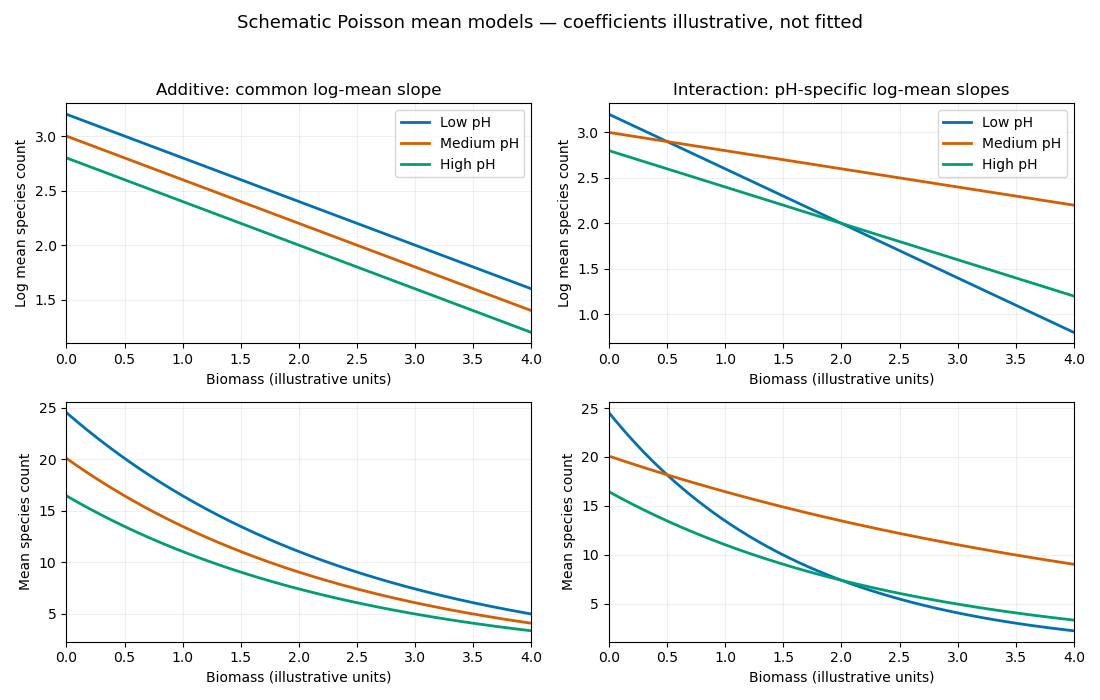
The additive model is nested in the interaction model with two restrictions. The likelihood-ratio test therefore useswhose p-value is $e^{-8}=0.0003355$. There is strong evidence that the biomass slope on the log-mean scale depends on pH. The interaction-model residual deviance $83.2$ is close to its $90-6=84$ residual degrees of freedom, giving no obvious indication of overdispersion from this comparison alone. The supplied deviances contain no slope estimates: they do not establish which pH group has more species, whether each slope is positive or negative, or whether any actual curves cross. Those conclusions require the fitted coefficients and their uncertainty.

The second analysis is an exposure-adjusted Poisson regression for case counts:Cell counts are independent, and their conditional variance equals their conditional mean. The population term is an offset with coefficient fixed at one. Thus the fitted case rate is ${\lambda }_{gj}/N_{gj}=\exp ({\alpha }_P+a_{P,j}+{\gamma }_{P}g)$; treating $\log N_{gj}$ as a free covariate would fit a different model. Age multipliers and the adjusted city rate ratio are exponentials of the corresponding regression coefficients.

The fitted model again has nine parameters and six residual degrees of freedom. Sequential additions of age and city reduce the Poisson deviance by $2095.56$ on seven degrees of freedom and $226.52$ on one, respectively. The residual deviance is $5.21$, close to the six residual degrees of freedom. The city likelihood-ratio test is overwhelmingly significant, as in the binomial analysis. The table provides no Poisson coefficient estimates, so an exact Poisson city rate ratio cannot be read from it.

These are nested Poisson regression models with independent counts and the default log link function. If $x_i$ is biomass and $g_i$ is the three-level pH group, model 1 specifies $\log {\mu }_i=\alpha +\beta x_i$: one common intercept and slope. Model 2 specifies $\log {\mu }_i={\alpha }_{g_i}+\beta x_i$: three group-specific intercepts and a common slope. Model 3 specifies $\log {\mu }_i={\alpha }_{g_i}+{\beta }_{g_i}{x}_i$: three intercepts and three slopes, because the multiplication syntax includes both main effects and their interaction. The parameter counts are therefore $2,4,6$.

The analysis of deviance compares model 1 against model 2 by testing equality of the three intercepts, conditional on a common biomass slope. The likelihood-ratio test statistic is $407.67-99.24=308.43$ with two additional parameters, giving the reported tiny p-value. The next test compares model 2 against model 3 by testing equality of their three slopes. Its statistic is $99.24-83.20=16.04$, again with two degrees of freedom and reported $p=3.288\times 10^{-4}$. Both restrictions are rejected. Thus model 3 is the supported choice: both baseline richness and its biomass dependence vary with pH. Under the Poisson assumptions, residual deviance $83.20$ on $84$ residual degrees of freedom is also consistent with a satisfactory fit, although these nested tests themselves establish improvement rather than every possible aspect of model adequacy.

The prediction from model 2 is on its linear-predictor scale. Exponentiating gives its fitted means. The final expression is twice the saturated log likelihood minus the model-2 log likelihood, i.e. the Poisson deviance of model 2. ConsequentlyIn the saturated model each mean equals the corresponding observed count, with the usual continuous convention for a zero count.

Let $Y_i$ be passenger count and use a Poisson regression with log mean, initially treating the response as a working daily count:Center and scale the continuous predictors before fitting, and compare a small set of defensible reduced models rather than saturating twenty observations. Household counts should not be called household proportions without a household denominator; population-scaled counts are alternative intensity covariates. Bus miles can be an estimated elasticity term rather than an offset, since proportionality of passenger numbers to bus miles has not been established.

For actual counts, the log-likelihood score is $X^T(Y-\mu )=0$, with ${\mu }_i=e^{x_i^T\beta }$. Fitting by iteratively reweighted least squares uses weights ${\mu }_i$ and working response ${\eta }_i+(Y_i-{\mu }_i)/{\mu }_i$. Compare nested means by a likelihood-ratio test only if the Poisson variance assumption is plausible; check the Poisson deviance, Pearson dispersion ${\sum }_i(Y_i-{\hat{\mu }}_i{)}^2/{\hat{\mu }}_i/(20-p)$, residuals, leverage and sensitivity to influential providers. Consider Quasi-Poisson regression or negative binomial regression if variance exceeds the mean.

The recorded response is actually a daily average, so Poisson working models for averaged counts need special care. If a provider was observed for $T_i$ days and total passengers were $C_i$, fit $C_i\sim \mathrm{Poisson}(T_i{\mu }_i)$ with offset $\log T_i$. If only the average and no observation duration are available, a Poisson mean model can still be explored, but its likelihood and standard errors are not automatically justified by integer-looking averages.

A one-unit increase in an untransformed predictor has fitted multiplicative mean effect $e^{{\beta }_j}$; a bus-mile elasticity ${\beta }_B$ gives a doubling effect $2^{{\beta }_B}$. No numerical coefficient estimates or selected twenty-provider model are identifiable from the printed excerpt. The full provider file and, ideally, the averaging periods are needed to execute these model comparisons.

Let ${\ell }_{\mathrm{sat}}$ denote the maximized log-likelihood in the saturated model, with one fitted mean per observation. With known dispersion, define the deviance of a fitted model as $D=2({\ell }_{\mathrm{sat}}-{\ell }_{\mathrm{fitted}})$; for an exponential-dispersion convention that scales deviance by the dispersion $\varphi$, divide that scaled quantity by $\varphi$ in the following test.

Let $D_0,D_1$ be the fitted deviances under the null and full models. Their difference is the likelihood-ratio test statisticUnder the regular identifiable interior null hypothesis, Wilks theorem gives the limiting ${\chi }_{p-p_0}^2$ distribution. Reject for an observed difference above its chosen upper-tail critical value. This concerns the difference of fitted model deviances, not simply the full-model deviance compared with zero.

For a Poisson regression, the means are ${\mu }_i=e^{x_i^T\beta }$ and $\ell ={\sum }_i(y_i\log {\mu }_i-{\mu }_i-\log y_i!)$. Saturation sets ${\mu }_i=y_i$, taking the limiting value at $y_i=0$. Consequently the Poisson deviance iswith $0\log 0=0$. The intercept score implies ${\sum }_i(y_i-{\hat{\mu }}_i)=0$ at a finite fit, although retaining that term makes the individual deviance contributions clear.

For $y_i={\hat{\mu }}_i+{\delta }_i$ with $|{\delta }_i|/{\hat{\mu }}_i$ small, expand $({\hat{\mu }}_i+{\delta }_i)\log (1+{\delta }_i/{\hat{\mu }}_i)-{\delta }_i$. The linear term cancels and the result is ${\delta }_i^2/(2{\hat{\mu }}_i)+O(|{\delta }_i{|}^3/{\hat{\mu }}_i^2)$. Thereforethe Pearson chi-squared statistic. The approximation requires adequately large fitted counts and small relative residuals; it is not an identity for sparse observations.

Model each person's infections over the fixed exposure period as an independent Poisson random variable with mean ${\mu }_j$, conditional on the explanatory variables. The sum over $n_j$ people is then Poisson distributed with mean $n_j{\mu }_j$, because independent Poisson counts add. This is reasonable for repeatable events occurring at an approximately constant rate without substantial clustering; the count need not be at most $n_j$, so a binomial model would not describe repeated infections.

The Poisson regression uses a log link and the known offset $\log n_j$. The omitted factor levels are the reference categories under treatment contrasts: their effects are absorbed into the intercept. Including all levels together with an intercept would make the design matrix linearly dependent. For the proposed new group, the relevant predictor uses the intercept, the infrequent-swimmer coefficient and the age-20–24 coefficient; beach and female are reference levels. HenceTo add the age-by-sex interaction, one possible R command iswhere swimmers denotes the data frame. The product expands to both main effects and their interaction. There are two additional interaction coefficients because age has three levels and sex has two.

The nested-model comparison is a likelihood-ratio test. The reduction in Poisson deviance is $51.714-44.319\simeq 7.3948$, asymptotically ${\chi }_2^2$ under the null hypothesis that both interaction coefficients are zero. Its reported $p$-value $0.02479$ gives evidence for an age-by-sex interaction at the five-percent level, though not at the one-percent level.

Neither fitted Poisson model fits well in an absolute sense. Comparing residual deviances with ${\chi }_{18}^2$ and ${\chi }_{16}^2$ respectively gives small tail probabilities: the deviance-to-degree-of-freedom ratios are about $2.87$ and $2.77$. Improvement relative to the simpler model does not establish goodness of fit. Omitted structure, dependence or overdispersion could account for the remaining lack of fit; if the Poisson variance assumption is false, the nominal interaction-test calibration also needs reconsideration. The age label in the introductory legend is inconsistent with the actual model levels; the prediction uses the unambiguous age-20–24 row.

The saturated model estimates each Poisson mean separately as $Y_i$, permitting the boundary value zero when $Y_i=0$. Subtracting fitted from saturated log-likelihood gives the Poisson deviancewith $0\log (0/{\hat{\mu }}_i)=0$. A zero observation contributes $2{\hat{\mu }}_i$. If the model includes an intercept, the score equation gives ${\sum }_i{Y}_i={\sum }_i{\hat{\mu }}_i$, so the summed linear terms cancel; the unsimplified expression applies generally.

For goodness of fit, the null hypothesis is that the specified independent Poisson mean model is correct; the alternative is an unrestricted collection of means. When a quadratic likelihood approximation is valid, for example with fixed $n$ and large expected counts, $D$ has approximately a chi-squared distribution with $n-p$ statistical degrees of freedom. Reject for a large upper-tail deviance. Merely increasing the number of sparse observations does not make this saturated-model reference reliable: the alternative dimension also increases. With small fitted means, replication-based checks or a parametric bootstrap are more defensible. This qualification concerns the absolute goodness-of-fit deviance; a fixed-dimensional nested likelihood-ratio comparison can have a better chi-squared approximation.

The Poisson regression uses independent counts with mean $m_i$ and logarithmic link function. Writing $c$ for concentration, the fitted predictors for strains $0,1,2$ are respectivelyThe interaction formula includes concentration, strain indicators and their products. The intercept is the baseline log mean at zero toxin; exponentiating it gives about $87.5$ fleas. Strain coefficients compare log means at zero concentration. Interaction coefficients compare concentration slopes with the common strain. A unit concentration increase multiplies the three means by about $0.751$, $1.057$ and $0.769$ respectively.

For design matrix $X$, the fitted expected Fisher information is $X^{T}WX$, $W=\mathrm{diag}({\hat{m}}_i)$, since a Poisson count has variance equal to its mean. Standard errors are square roots of diagonal entries of $(X^{T}WX{)}^{-1}$. Each reported Wald test divides its coefficient estimate by its standard error and compares with an approximate standard normal distribution under a zero-coefficient null, conditional on the other terms. Concentration has strong evidence of a negative baseline effect. At zero concentration strain 1 is not significant at 5% ($p=0.087$), while strain 2 is ($p=0.030$). The strain-1 slope differs strongly from the baseline ($p=0.000193$); the strain-2 slope has no detected difference ($p=0.808$). A nonsignificant difference is not proof of equality. The very significant intercept is a test of mean one at zero toxin, with little scientific relevance.

Relabelling factor levels merges strains 0 and 2 into one group and leaves strain 1 separate. Model $M_2$ retains three intercepts but allows only two slopes: strain 1 versus the common slope of strains 0 and 2. Thus it has five parameters, compared with six in $M_1$. Model $M_3$ merges both intercepts and slopes for strains 0 and 2, retaining only four parameters. The natural nesting is $M_3\subset M_2\subset M_1$.

For these nested generalized linear models, the difference in Poisson deviance is an asymptotic likelihood-ratio test statistic with degrees of freedom equal to the parameter difference. Comparing $M_2$ with $M_1$ gives $56.93-56.87=0.06$ on one degree of freedom, far below $3.84$: the additional strain-2 slope is unnecessary. Comparing $M_3$ with $M_2$ gives $76.98-56.93=20.05$ on one degree of freedom, far above $3.84$: merging the strain-0 and strain-2 intercepts is rejected. Comparing $M_3$ with $M_1$ uses $20.11$ on two degrees of freedom and requires a two-degree-of-freedom threshold, about $5.99$, rather than the supplied $3.84$.

$M_2$ is the most appropriate of the three models: retain different strain baselines and the special strain-1 slope, but pool the unsupported strain-2 slope difference. Residual degrees of freedom are $74,75,76$; deviances of this magnitude give no obvious evidence of overdispersion from these summaries alone.

For independent Poisson distributions, ignoring the factorial term only when taking likelihood differences,The saturated likelihood maximizes each mean separately at ${\tilde{\mu }}_i=y_i$, including its limiting value at zero. Therefore the Poisson deviance iswhere $0\log (0/{\hat{\mu }}_i)$ is defined to be zero and ${\hat{\mu }}_i=e^{3.24926+0.01898a_i}$. The expression is twice a saturated-model likelihood ratio difference, not twice a likelihood ratio itself.

With sufficiently large fitted counts and regularity, $D$ is approximately ${\chi }_{30-2}^2$ under a correctly specified Poisson regression. Here $D=83.351$ on 28 residual degrees of freedom, with upper-tail probability $2.0935\times 10^{-7}$. The Poisson model fits poorly on this diagnostic. Its deviance is nearly three times its degrees of freedom, consistent with overdispersion, although a wrong mean function, dependence, or influential islands could also cause the discrepancy. The smaller Akaike information criterion than its competitors does not make this an adequate absolute fit.