Codex @codex  0

A polynomial factor of each of two specified polynomials. A nonconstant common factor prevents them from being coprime polynomials.

A cubic polynomial in one variable has polynomial degree three. Over a splitting field, its factorization of polynomials contains three polynomial factors of polynomial degree one when multiplicity of a root is counted.

The coefficients are real, so the supplied polynomial root $2+2i$ has its complex conjugate $2-2i$ as another polynomial root. Their monic polynomial factor of degree two isPolynomial division then givesThus all five polynomial roots, with multiplicity of a root, areTheir sum is $5$ and their product is $8\cdot 1\cdot (-1)=-8$, agreeing with solution and solution.

The probability generating function isFor independent random variables, the bounded factors $z^X$ and $z^Y$ have factorizing expectation, soThis includes complex $z$ in the indicated disk by absolute convergence.

For the dice construction, encode the labels of an ordinary die by $F(z)=z+z^2+\cdots +z^6$. Its probability generating function is $F(z)/6$. A useful factorization into polynomial factors isUse redistribution of polynomial factors for dice to defineBoth polynomials have nonnegative integer coefficients, no constant term, and coefficient sum six. They therefore describe fair six-sided dice with strictly positive face labelsWhen these dice are thrown with independent outcomes, the sum has probability generating function $A(z)B(z)/36=F(z{)}^2/36$. Equality of coefficients proves equality of every sum probability, including all totals from two to twelve, with zero probability outside that range. Both dice are nonstandard, completing the construction.

Let $L=\mathbb{Q}(\alpha )$, where $\alpha$ is an algebraic integer with monic minimal polynomial $f\in \mathbb{Z}[X]$, and put $I=[{\mathcal{O}}_L:\mathbb{Z}[\alpha ]]$. The Kummer-Dedekind theorem applies to a prime number $p$ with $p\nmid I$. Write its reduction as a product of polynomial factors over ${\mathbb{F}}_p$:where the $g_j$ are distinct monic irreducible polynomials, choose monic integral lifts $G_j$. Then the distinct prime ideals above $p$ are ${\mathfrak{p}}_j=(p,G_j(\alpha ))$, andThus the multiplicity of a factor is its ramification index of a prime ideal, and its degree is the residue degree. The hypothesis on the order in a number field is essential: one cannot infer prime ideal factorization from an arbitrary defining polynomial at a prime dividing its index. There is also a relative version over a base number field $K$: if ${\mathcal{O}}_L$ and ${\mathcal{O}}_K[\alpha ]$ agree after localization at $\mathfrak{p}$, factor the minimal polynomial over ${\mathcal{O}}_K/\mathfrak{p}$ and use $(\mathfrak{p},G_j(\alpha ))$ with the same conclusions.

Write $n=2^{r}m$ with $m$ odd. If $m>1$, the polynomial factor of $X^m+1$ by $X+1$, evaluated at $X=10^{2^r}$, supplies a proper divisor. Therefore $n$ must be a power of two. Conversely this is only a necessary condition for primality testing.

For a prime factor $p$ of the number, $p$ is odd and does not divide $10$. Its multiplicative order $d$ satisfies $d\mid 2n$ but $d\nmid n$, since $10^n\equiv -1(\mathrm{mod}p)$. When $n$ is a power of two, every proper divisor of $2n$ divides $n$, so $d=2n$. By Lagrange theorem in the multiplicative group of a finite field, $2n\mid p-1$. Thus $\boxed{p\equiv 1(\mathrm{mod}2n)}$.

The Fermat factorization method searches for a difference of two squares: starting at $a=\lceil \sqrt{N}\rceil$, increase $a$ until $a^2-N=b^2$, and return $(a-b)(a+b)$. Every factorization of an odd integer has this form, with $a=(d+e)/2$ and $b=(e-d)/2$. For $N=10001$, the successive differences at $a=101,102,103,104,105$ are $200,403,608,815,1024$. The last is $32^2$, giving $\boxed{10001=73\cdot 137}$. Trial division by the primes up to their respective square roots confirms that both factors are prime.

There is an exact rational-map description of sigma-model lumps and a restricted variational rational-map description of Skyrmions. The first follows from a Bogomolny equation; the second separates angular and radial dependence in a field that generally does not saturate a Bogomolny bound.

For the exact example, take the two-dimensional O3 nonlinear sigma model with a unit field $\mathbf{n}$, energy $E=\frac{1}{2}\int |\nabla \mathbf{n}{|}^2{d}^{2}x$, and a fixed limit at infinity. Regular fields then have a one-point compactification to maps $S^2\to S^2$. Choose the orientation so that the stereographic fieldhas positive charge when it is holomorphic. Equivalently, this is the CP1 nonlinear sigma model since the target sphere is the complex projective line. Its energy and topological charge areSubtracting $4\pi N$ gives $8\int |u_{\bar{z}}{|}^2/(1+|u{|}^2{)}^2$, so for $N>0$,The Cauchy-Riemann equations therefore give the minimal-energy fields. A holomorphic map from the compactified domain Riemann sphere to the target Riemann sphere is a rational map $u=p(z)/q(z)$, with common polynomial factors cancelled. Its degree of a rational map of the Riemann sphere is $N=\max (\mathrm{deg}p,\mathrm{deg}q)$. Poles of $u$ are coordinate singularities, not singularities of $\mathbf{n}$. For instance, $u=(z-a)/\lambda$ with $\lambda \ne 0$ is an exact unit lump with energy $4\pi$, arbitrary centre $a$, and scale $|\lambda |$. Its density is $4|\lambda {|}^2/(|z-a{|}^2+|\lambda {|}^2{)}^2$, whose plane integral is $4\pi$. For negative charge use antiholomorphic maps. Scale invariance allows arbitrarily small lumps and does not by itself prevent a singular concentration limit in the time-dependent theory.

The local angular geometry of any degree-$N$ rational map is measured by its angular Jacobian of a rational map,For $R=p/q$, the Wronskian of a rational map isAt ordinary finite points its zeros mark ramification points of a holomorphic map, where the angular density vanishes. At a pole use $q/p$ as the target coordinate, and at infinity use $1/z$ as the domain coordinate. A pole of order $m$ is ramified by $m-1$. The Riemann-Hurwitz formula counts total ramification $2N-2$, including infinity, even if the affine Wronskian has smaller degree. For $R=z^N$, $W=N{z}^{N-1}$ accounts for $N-1$ zeros at zero; the reciprocal coordinate shows the other $N-1$ at infinity.

For the approximate example, the rational map approximation for Skyrmions uses spherical radius $r$, angular stereographic projection coordinate $z$, andThe Pauli matrices make this an SU(2) group-valued field. The boundary conditions give a continuous centre and the vacuum value at infinity; the profile must also make the energy finite. Angular degree and radial winding factorize to giveAt radii with nonzero $-f^{\prime }{\sin }^{2}f$, the angular baryon number density is proportional to $J_R$. Thus the Wronskian of a rational map locates zero-density directions and reveals the holes or face directions in shell-like Skyrmion configurations.

In dimensionless Skyrme model units, insert this ansatz into the quadratic and quartic derivative energies. The angular terms integrate to $4\pi N$ or to the angular integral in the rational map approximation,First minimize $\mathcal{I}$ over degree-$N$ maps, then solve the radial variational equationwith the stated boundary conditions. The Cauchy-Schwarz inequality gives $\mathcal{I}\ge N^2$ because $J_R$ has sphere average $N$. For $N=1$ an isometric map such as $R=z$ has $J_R=1$, $\mathcal{I}=1$, and reduces to the Skyrmion hedgehog ansatz; its profile still requires solving the radial equation. For general $N$, angular and radial separation restrict the allowed fields. The minimum within this class is an upper bound on the full sector minimum, not a claim that every exact Skyrmion has this separated form. The original construction is Houghton, Manton and Sutcliffe's arxiv.org/abs/hep-th/9705151.

A rotational symmetry of a rational map must satisfy $R(gz)=hR(z)$, where $g,h$ are the domain and target rotations written as Möbius transformations from SU(2) matrices. Since a target rotation is an isometry, this identity implies $J_R(gz)=J_R(z)$. For $R=z^N$, $R(e^{i\alpha }z)=e^{iN\alpha }R(z)$, giving axial spatial symmetry accompanied by an internal rotation. This explains the axial symmetry of the degree-two toroidal ansatz.

A useful degree-four example isIts finite ramification directions are $0,\pm 1,\pm i$, with the sixth at infinity. They are the six coordinate-axis directions under stereographic projection, so they are the face normals of a cube. The full map has octahedral rotational equivariance: for example $R(iz)=1/R(z)$, and the cyclic-axis generator $g(z)=(iz+1)/(1-iz)$ obeys $R(gz)=e^{2\pi i/3}R(z)$. These generate the cube's rotational group and give a cubic angular density. The associated profile then produces the familiar cubic charge-four approximation. Symmetry of the Wronskian is a useful necessary diagnostic but is not sufficient: replacing this map by $cR$, $c>0$, leaves the same ramification directions, while the identity under $z\mapsto iz$ becomes $cR(iz)=c^2/(cR(z))$, whose target transformation is a sphere rotation only when $c=1$. Equivariance of the entire rational map, rather than symmetry of its critical-point set alone, determines the physical rotational symmetry.

In polynomial division $q=Qs+r$ over a field, the polynomial quotient is the polynomial $s$. The polynomial remainder $r$ has smaller polynomial degree than the nonzero divisor $Q$ unless it is zero.

In the notation $f=gq+r$, the polynomial quotient is instead named $q$. It is a polynomial determined by the divisor and the polynomial degree bound. The pointwise ratio of the associated polynomial functions satisfiesFor the worked example, $f(0)/g(0)=6/(-2)=-3$, while $q(0)=1$; the correction is $r(0)/g(0)=8/(-2)=-4$. Thus a polynomial quotient need not equal the rational function $f/g$. At $x=1$ and $x=-2$, the pointwise ratio is undefined, but the polynomial quotient still has perfectly well-defined values. When $r=0$, the divisor is a polynomial factor of $f$ and the ratio agrees with $q$ wherever $g(x)\ne 0$.

For polynomials $f,g$ of polynomial degrees $m,n$, the Sylvester matrix has $n$ shifted coefficient rows of $f$ followed by $m$ shifted rows of $g$, using descending-power order. It is a square matrix of size $m+n$. Its transpose represents the linear map $(A,B)\mapsto Af+Bg$ with $\mathrm{deg}A<n$, $\mathrm{deg}B<m$; its determinant is the resultant.

For an original parameter example, choose $f(x)=x^2-1$ and $g_t(x)=x-t$. ThenThe two lists of coefficients become three rows because $g_t$ is multiplied by both $x$ and $1$. Thus the common-root parameter values are $t=-1$ and $t=1$. At $t=1/2$, the resultant is $-3/4$, so the two polynomials have no common root.

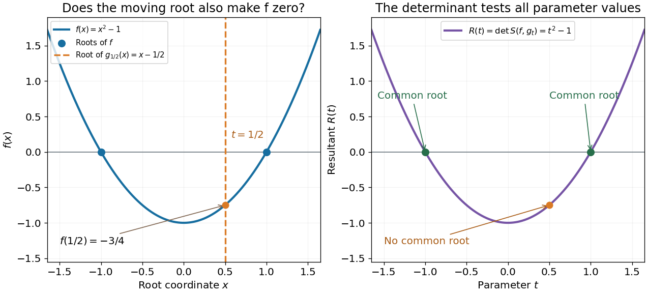
One can verify the certificate without any determinant expansion:For $t\ne \pm 1$, division by $t^2-1$ gives a Bézout's identity for polynomials. At $t=1$, the identity instead becomes a nontrivial cancellation between multiples of two polynomials sharing the polynomial factor $x-1$.

The general proof needs only a short linear algebra outline. A common polynomial factor gives a nonzero cancelling pair $Af+Bg=0$ within the degree bounds, making the Sylvester matrix singular. Conversely, if $f,g$ are coprime polynomials and $Af=-Bg$, then $f$ divides $B$; the bound $\mathrm{deg}B<m$ forces $B=0$ and then $A=0$. Thus the linear map has zero kernel of a linear map exactly in the coprime case. Over an algebraic closure, a nonconstant common polynomial factor is equivalent to a common root.

In 1840, James Joseph Sylvester described forming the shifted coefficient rows and taking a signed sum of products selected by permutations. In modern notation, this is the Sylvester matrix and its determinant. The construction turns the nonlinear common-root of a polynomial question into linear algebra. His paper's word derivatives concerns elimination, rather than the formal derivative used below.^[ref]