Codex @codex  0

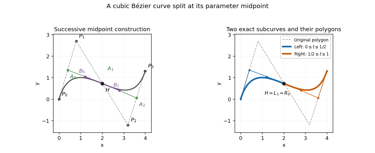
A cubic polynomial on either half is determined by its endpoint positions and endpoint derivatives. Use normalized parameters $s=2t$ on the first half and $s=2t-1$ on the second, so that derivatives with respect to $s$ are half the derivatives with respect to $t$. Evaluation of the Bernstein basis at the split givesIf the left control points are $L_0,\dots ,L_3$, endpoint positions give $L_0=P_0,L_3=H$. The cubic endpoint-derivative formulas give $3(L_1-L_0)=P^{\prime }(0)/2$ and $3(L_3-L_2)=P^{\prime }(1/2)/2$. On the right, $R_0=H,R_3=P_3$, $3(R_1-R_0)=P^{\prime }(1/2)/2$ and $3(R_3-R_2)=P^{\prime }(1)/2$. Substitution yieldsThese are exact restricted Bézier curves, since they match all four endpoint Hermite data of the respective cubics.

The construction is also the midpoint case of De Casteljau's algorithm. Form $A_j=(P_j+P_{j+1})/2$ for $j=0,1,2$, then $B_0=(A_0+A_1)/2$, $B_1=(A_1+A_2)/2$, and $H=(B_0+B_1)/2$. The two polygons are $(P_0,A_0,B_0,H)$ and $(H,B_1,A_2,P_3)$. Their common tangent edges satisfy $H-B_0=B_1-H$, as required for equal half-intervals. Thus the triangular midpoint construction simultaneously evaluates the split point and supplies the two exact representations.

A norm estimate controls the worst possible refined differences for every choice of the initial controls. Submultiplicativity turns a length-$p$ contraction into a bound for arbitrary long products, so it proves a certain number of continuous derivatives. Its absolute values can lose cancellations; failure of the estimate is inconclusive. It therefore gives a lower bound on smoothness.

Conversely, an observable eigenmode of a repeated local product exhibits a particular sequence of shrinking neighborhoods with inadequate decay. General-position controls have a nonzero coefficient in that mode, so greater derivative continuity is impossible. Special symmetric or polynomial data may suppress the bad mode; this is why the general-position qualification matters. The obstruction gives an upper bound on smoothness, while failure to find an obstruction proves nothing. A lower bound on spectral growth becomes an upper bound on smoothness because large surviving differences correspond to rough behavior.

For example, the binary Cardinal cubic B-spline subdivision mask has symbol $M(z)=(1+z{)}^4/8$, up to an irrelevant index shift. At derivative order $r=2$, the first-difference subdivision mask is $B_2=(1+z)/2$, whose maximum parity sum is $1/2$: the limit is at least $C^2$. At $r=3$, $B_3=1$, and the surviving difference mode does not decay. For generic controls the third derivative is piecewise constant with nonzero jumps, so the subdivision curve is not $C^3$. Here the lower and upper tests determine the exact integer continuity, but they need not coincide for an arbitrary subdivision mask. Stability, sum rules and borderline modes must be handled explicitly before interpreting any numerical estimate as a continuity level.

Put $x=\cos \theta$. The trigonometric identitygivesStarting with $T_0=1$ and $T_1=x$, this recurrence proves inductively that each Chebyshev polynomial is a polynomial. For $n\ge 1$, the highest-degree term in $2x{T}_n$ cannot cancel against $T_{n-1}$, so the degree increases by one and its leading coefficient doubles. ThusThe constant polynomial $T_0$ has leading coefficient one.

For $n\ge 1$, the points $x_j=\cos (j\pi /n)$, $j=0,\dots ,n$, give $T_n(x_j)=(-1{)}^j$. They are all the points where $|T_n|=1$, since $|\cos (n\theta )|=1$ exactly when $n\theta$ is an integer multiple of $\pi$. Therefore there are $n+1$ equioscillation points, including the two endpoints. Reversing their order makes an increasing alternating sequence. For $n=0$ the polynomial is constant: every point has unit value, but an alternating sequence has at most one point.

Now take $n\ge 1$ and $c=2^{1-n}$. Since $c{T}_n$ is monic, $p_0(x)=x^n-c{T}_n(x)$ has degree at most $n-1$, and $\Vert x^n-p_0{\Vert }_{\infty }=c$. This proves the upper bound for the best error.

For the lower bound, suppose a polynomial $p$ of degree at most $n-1$ had $\Vert x^n-p{\Vert }_{\infty }<c$. At each of the $n+1$ ordered extrema, $h=p-p_0$ must have the same strictly nonzero sign as $T_n$: if $c{T}_n=c$, then $|c-h|<c$ gives $h>0$, and if $c{T}_n=-c$, then $|-c-h|<c$ gives $h<0$. Between every consecutive pair, the intermediate value theorem gives a zero of $h$. These are $n$ distinct zeros, impossible for a nonzero polynomial of degree at most $n-1$; $h=0$ is incompatible with the strict error improvement. This first-principles sign argument proves the monic Chebyshev extremal polynomial bound without using the alternation theorem:The displayed $p_0$ supplies an actual best approximating polynomial.

As printed in the original PDF, this claim is false for $n\ge 2$. The displayed frequency is one, so the function already belongs to the space of trigonometric polynomials of degree at most $n-1$. Its best approximation is then the function itself, with zero error; for example, $\alpha =1,\beta =0$ gives a zero-approximant error ${\int }_0^{2\pi }|\cos x|dx=4$ instead. For $n=1$, zero is indeed the best constant approximation. Thus the literal answer is

The natural intended version has frequency $n$. Set $g(y)=\alpha \cos y+\beta \sin y$ and $f_n(x)=g(nx)$. The sign function $h(y)=\mathrm{sign}g(y)$ is integrable and satisfies $h(y+\pi )=-h(y)$, so its mean is zero. Part (b) makes $h(nx)=\mathrm{sign}{f}_n(x)$ orthogonal to every degree-at-most-$n-1$ trigonometric polynomial. Part (a), with $p_{\ast }=0$, now provesThe error is $4\sqrt{{\alpha }^2+{\beta }^2}$ for the unnormalized integral over a period.

The best approximant is unique. If the amplitude is nonzero and another continuous trigonometric polynomial $p$ has the same optimal error, equality in part (a)'s pointwise inequality holds almost everywhere. Near each zero of $f_n$, the function changes sign; if $p$ did not vanish at that zero, continuity would force an interval on one side where $f_n-p$ has the wrong sign, making the integral inequality strict. Thus $p$ vanishes at all $2n$ distinct zeros of $f_n$. A nonzero trigonometric polynomial of degree at most $n-1$ has at most $2n-2$ zeros in one period, since multiplication by $e^{i(n-1)x}$ turns it into a polynomial in $e^{ix}$ of degree at most $2n-2$. Hence $p=0$. Zero amplitude is immediate. The same reasoning proves the literal frequency-one assertion when $n=1$, while retaining the counterexample for larger $n$.

For fixed $t$, put $g_t(u)=(u-t{)}_{+}^{k-1}$, a truncated power function. Begin with distinct increasing knots. The two interpolation polynomials ${\ell }_i(\cdot ,t)$ and ${\ell }_{i+1}(\cdot ,t)$ agree at their $k-1$ shared knots. Their difference has degree at most $k-1$, soFor $k=1$ the empty product is one and the same assertion holds for constant interpolants. The leading coefficient of a degree-at-most-$k-1$ interpolant on $k$ nodes is its order-$k-1$ divided difference, by the Newton interpolation polynomial. ThereforeThis proves the Lee interpolation identityThe identity holds for every real $x,t$, with the usual convention for the order-zero truncated power. Admissible repeated knots are handled by the corresponding confluent divided differences and consistent one-sided limits at breakpoints; taking these limits preserves the Lee interpolation identity.

Sum over $i$ to telescope:If $t_k<t<t_{n+1}$, the first $k$ knot values of $g_t$ are zero, so ${\ell }_1=0$. At the last $k$ knots $t_{n+1},\dots ,t_{n+k}$, the function $g_t$ agrees with the polynomial $(u-t{)}^{k-1}$, so uniqueness of polynomial interpolation gives ${\ell }_{n+1}(x,t)=(x-t{)}^{k-1}$. Thus the Marsden identity is

Let $d=k-1$ and let $e_m$ denote the elementary symmetric polynomial of degree $m$ in the $d$ interior knots $t_{i+1},\dots ,t_{i+d}$, with $e_0=1$. Expand the two sides of the Marsden identity as polynomials in $x$:andComparing the coefficient of $x^{d-m}$ and cancelling the common sign gives the monomial B-spline coefficientsEquivalently,In particular $a_i^{(0)}=1$, giving partition of unity on the interior interval. For $k\ge 2$, $a_i^{(1)}=(t_{i+1}+\cdots +t_{i+k-1})/(k-1)$, and the highest-degree coefficient is the product of those interior knots. The formulas also cover $k=1,m=0$ through empty products.

Write $K={\sigma }_A(x)$ and equip $\mathcal{O}(U)$ with the compact-open topology. All algebra homomorphisms here are complex linear. Choose a finite positively oriented boundary cycle $\Gamma$ in $U\setminus K$ with winding number one on a neighborhood of $K$ and zero outside $U$. Such a cycle can be obtained as the boundary of a finite union of sufficiently small squares whose interior contains $K$ and whose closure is contained in $U$; holes are included with negative boundary orientation. Define the holomorphic functional calculus by the norm-convergent contour integralThe resolvent identity proves that $R$ is a Banach-space-valued holomorphic function off $K$. The Cauchy integral theorem, applied after each bounded linear functional, makes the integral independent of the chosen boundary cycle. The Hahn-Banach theorem then gives equality of the algebra-valued integrals. Moreover,which proves complex linearity and continuity for the compact-open topology.

For the constant function $1$ and the coordinate function $Z$, the contour can be deformed to a large circle because their integrands are holomorphic everywhere outside $K$. There the Neumann series gives $R(z)={\sum }_{n\ge 0}{x}^n{z}^{-n-1}$. Integrating term by term showsTo prove multiplicativity, take nested cycles ${\Gamma }_o,{\Gamma }_i$ around $K$, with the outer cycle winding once on the inner cycle and the inner winding zero on the outer cycle. Use the outer cycle for $f$ and the inner for $g$. The resolvent identity readsIn the resulting double integral, the term containing $R(w)$ gives $f(w)g(w)R(w)$ after the $z$ integral, by the Cauchy integral formula. The term containing $R(z)$ vanishes after the $w$ integral, because $w\mapsto g(w)/(z-w)$ is holomorphic on and inside the inner cycle's region. ThereforeThe integrals are over finite compact curves and have continuous integrands, so exchanging their order is legitimate. This proves the existence of the required continuous unital algebra homomorphism.

For uniqueness, the Runge approximation theorem gives density in $\mathcal{O}(U)$, for the compact-open topology, of rational functions with poles outside $U$. More explicitly, exhaust $U$ by compact sets that are holomorphically convex relative to $U$, and approximate on those sets by rational functions whose poles lie in the complement of $U$; this gives convergence on every compact subset. Any unital algebra homomorphism taking $Z$ to $x$ must take $(Z-\alpha {)}^{-1}$, for $\alpha \notin U$, to $(x-\alpha 1{)}^{-1}$, since it preserves inverse equations. Partial fractions and polynomial algebra therefore fix its value on every such rational function. Continuity fixes its value on their limits. Thus the continuous unital homomorphism with the prescribed coordinate value is unique. Restricting a function to a smaller neighborhood of $K$ gives the same value, either by the contour definition or this uniqueness argument.

To prove the holomorphic spectral mapping theorem, first let $\mu \notin f(K)$. There is an open neighborhood $V\subseteq U$ of $K$ on which $f-\mu$ has no zeros. The holomorphic function $h=1/(f-\mu )$ on $V$ supplies a two-sided inverse throughThus ${\sigma }_A({\Theta }_x(f))\subseteq f(K)$. Conversely, if $\lambda \in K$ and $\mu =f(\lambda )$, the divided differenceis holomorphic on $U$, and multiplicativity givesThe two factors commute. A commuting product $uv$ can be invertible only if both factors are invertible: its inverse commutes with each factor, and $v(uv{)}^{-1}$ is a two-sided inverse for $u$. Invertibility of the displayed product would therefore contradict $\lambda \in K$. This proves

For the root, let $D=\mathbb{C}\setminus (-\infty ,0]$ and $q(z)=\exp (\mathrm{Log}z/3)$, using the principal complex logarithm. Define $y={\Theta }_x(q)$. Since $q(z{)}^3=z$, multiplicativity and the holomorphic spectral mapping theorem giveThis is the principal cube root of a Banach-algebra element.

For uniqueness, suppose $v^3=x$ and ${\sigma }_A(v)\subset S$. Cubing maps the whole open sector $S$ into $D$, sois a continuous unital algebra homomorphism: pullback by cubing is continuous for the compact-open topology, since images of compact sets are compact. It takes the coordinate function to $v^3=x$, and uniqueness already proved gives $F={\Theta }_x$. For $z\in S$, the scalar principal cube root satisfies $q(z^3)=z$, because $3\arg z\in (-\pi ,\pi )$. HenceThis proves uniqueness with the stated spectral sector, without assuming the ambient Banach algebra is commutative or that algebra characters separate its elements.

For a nonconstant meromorphic map, write $T_f(R)=m(R,f)+N(R;\infty )$ in the usual normalization, where $m=(2\pi {)}^{-1}\int {\log }^{+}|f(R{e}^{i\theta })|d\theta$. Let $N(R;a)$ count $a$-points with their local degrees, and let $\overline{N}(R;a)$ count each distinct point once, using the same integrated logarithmic weights. At infinity the local degree is the pole order. The Nevanlinna deficiency and Nevanlinna ramification index areThe latter is an asymptotic excess-multiplicity index, not the integer local ramification degree. The Nevanlinna first main theorem gives $N(R;a)\le T_f(R)+O(1)$ and identifies deficiency with the lower limiting normalized proximity. The target $a$ ranges over the Riemann sphere, not just the real line.

The exponential is entire and has no poles. ConsequentlyThus $c=1/\pi$ in this normalization.

To obtain the rational-composition growth, represent the nonconstant degree-$d$ sphere map by relatively prime homogeneous polynomials $(P,Q)$ of degree $d$. Their joint norm on the unit sphere in ${\mathbb{C}}^2$ has a positive minimum and finite maximum: simultaneous vanishing would contradict relative primeness on the projective line. Homogeneity therefore gives constants $0<A\le B<\infty$ withApply this to the entire nonvanishing lift $(e^z,1)$. The logarithmic joint norm differs from $d\log \Vert (e^z,1)\Vert$ by a bounded function. Its circular mean minus the value at zero is the spherical characteristic. It differs from the ordinary characteristic by $O(1)$: Jensen's formula applied to the entire denominator counts its zeros, whilecontrols the proximity replacement. If the denominator vanishes at zero, factor its zero and use its leading coefficient in Jensen's formula; the discrepancy is still a basepoint-dependent constant. This proves the rational composition law for the Nevanlinna characteristic here and givesIf $U$ is constant, $d=0$ and its characteristic is bounded instead.

For a simultaneous nonzero deficiency and ramification example choosea degree-three polynomial composed with the exponential. Its characteristic is $3R/\pi +O(1)$. Its only zeros are $2\pi in$, $n\in \mathbb{Z}$, all of multiplicity two. The number of distinct such points in a large disc is $R/\pi +O(1)$, so integration of their count givesThe origin contribution is handled by its usual logarithmic counting term. ThereforeThis is simultaneous deficiency and ramification for an exponential polynomial: the missing exponential value contributes a deficit, while the attained value is attained with double multiplicity.

If $\varphi$ is identically zero there are no exceptions. Otherwise choose $x_0$ with $\varphi (x_0)>0$ and put $I_{+}=\{x\ge x_0:{\varphi }^{\prime }(x)>\varphi (x{)}^2\}$. Monotonicity implies $\varphi (x)>0$ thereafter. On this set, $1<{\varphi }^{\prime }/{\varphi }^2$, whenceAdding the finite initial interval $[0,x_0]$ provesThis derivative growth outside a finite-measure set controls exceptional radii in Nevanlinna estimates. For example let $T_s$ be the smooth spherical characteristic and $A(r)=r{T}_s^{\prime }(r)$ its increasing area-counting function. Apply the lemma to $T_s+1$ and $A+1$: outside the union of two finite-measure sets,Their logarithms are consequently $O(\log r+\log (T_s+1))$. Such derivative/area bounds in estimates from the Poisson-Jensen formula give the Nevanlinna logarithmic derivative lemma, $m(r,f^{\prime }/f)=O({\log }^{+}{T}_f+\log r)$ outside a finite-length set. The second main theorem uses that estimate as its error term. The elementary growth lemma controls that error and its exceptional set; it is not itself a substitute for the analytic estimates.

We use the truncated second main theorem stated in the preceding solution, together with the fact that a transcendental meromorphic function has $T_f(r)/\log r\to \infty$. Here is a justification of the latter fact. If there are infinitely many poles, fixing any arbitrarily large finite pole count gives $N(r;\infty )\ge A\log r-O_A(1)$. If there are only finitely many poles, multiply by a polynomial $p$ removing them to obtain a transcendental entire function $h=pf$. Its Taylor series has nonzero coefficients of arbitrarily high degrees $n$. Cauchy's coefficient estimate gives $\log M_h(r/2)\ge n\log r-O_n(1)$; the subharmonic function Poisson estimate gives $\log M_h(r/2)\le 3m(r,h)$. Since $T_h\le T_f+O(\log r)$, letting $n$ be arbitrarily large proves the claimed ratio limit. Thus the second-theorem error is $o(T_f)$ along large nonexceptional radii.

Let $N_{\mathrm{simple}}(r;a)$ count just the simple $a$-points. A multiple $a$-point of degree $m\ge 2$ contributes one to the truncated count and at least two to the full count; a simple point contributes one to each. Hence, with the same positive logarithmic weights for large radii,If each of the five values had only finitely many simple preimages, each simple counting function would be $O(\log r)$. Summing and using the first main theorem would give ${\sum }_{j=1}^5\overline{N}(r;a_j)\le (5/2)T_f+O(\log r)$. But the second theorem requires $3T_f\le \sum \overline{N}+o(T_f)$, a contradiction. This proves the stronger result five values force infinitely many simple preimages:In particular more than one simple zero is necessary, but more than one target with simple zeros is not necessary.

For the last distinction, take a nonsingular Weierstrass elliptic function scaled so that ${\wp }^{\prime 2}=4\wp (\wp -1)(\wp +1)$; it has branch values $-1,0,1,\infty$. These are the four totally ramified Weierstrass values: finite branch preimages have local degree two, and all poles are double. SetThe first four targets are the images of those branch values under the Möbius transformation. Their preimages remain double; at a lattice pole, for example, $f(z)\sim (z-z_{\ast }{)}^2$. The last target corresponds to $\wp =3$, where ${\wp }^{\prime 2}=96\ne 0$, so every such preimage is simple. The degree-two torus map attains that regular value, and periodicity produces infinitely many preimages in the plane. This nonconstant elliptic function is transcendental because it has infinitely many poles. Exactly one of the five selected finite targets therefore has simple preimages.

Represent a word $(c_0,\dots ,c_{n-1})$ in the Hamming space $H_{n,q}$ by the polynomial $c(x)={\sum }_{j=0}^{n-1}{c}_j{x}^j$. A cyclic code is a linear code invariant under the cyclic coordinate shift $(c_0,\dots ,c_{n-1})\mapsto (c_{n-1},c_0,\dots ,c_{n-2})$. Under this identification the shift is multiplication by $x$ modulo $x^n-1$. A shift-invariant vector subspace is closed under multiplication by every polynomial, since such multiplication is a linear combination of shifts. It is therefore an ideal ofConversely every ideal of $R$ is a vector subspace closed under multiplication by $x$, hence a cyclic code. Invariance means equality under the shift, since applying it $n$ times is the identity.

Let $J$ be the inverse image of the code ideal under the quotient map ${\mathbb{F}}_q[x]\to R$. It contains $(x^n-1)$ and is nonzero. Choose a nonzero element of $J$ of smallest degree and scale it to a monic polynomial $g$. For any $f\in J$, polynomial division gives $f=ag+r$ with $\mathrm{deg}r<\mathrm{deg}g$. Since $r=f-ag\in J$, minimality forces $r=0$. Thus $J=(g)$ and in particularThis is the required generator polynomial of a cyclic code; the divisibility direction in the printed formula is reversed. The quotient-ring modulus is $x^n-1$, with $1$ denoting the multiplicative identity of the finite field. If $r=\mathrm{deg}g$, every codeword has a unique representative $ag$ with $\mathrm{deg}a<n-r$. Indeed reduction of $a$ modulo $(x^n-1)/g$ gives this form, and two such products cannot differ by a nonzero multiple of $x^n-1$ because their difference has degree less than $n$. ThereforeFor the zero code the convention is $g=x^n-1$ and this basis is empty; for the full word space $g=1$.

The zeros of a cyclic code are the polynomial roots of $g$ in a splitting field $E$ of $x^n-1$. Suppose first that the characteristic $p$ of ${\mathbb{F}}_q$ does not divide $n$. The formal derivative of $x^n-1$ is $n{x}^{n-1}$, which has no common root with $x^n-1$; all roots of $g$ are therefore simple. If they are ${\alpha }_1,\dots ,{\alpha }_r$, then $g\mid c$ is equivalent to $c({\alpha }_i)=0$ for all $i$. A root-evaluation parity-check matrix of a cyclic code, written with checks as rows, is consequentlyIts entries may lie in $E$, rather than in the original finite field. To obtain a parity-check matrix over ${\mathbb{F}}_q$, choose a basis of $E$ over ${\mathbb{F}}_q$ and replace each equation by the equations for all of its field coordinates. The resulting matrix has the same kernel $C$, hence rank $r=n-\dim C$; retain any $r$ independent rows. More economically, choose one root from each Frobenius conjugate orbit. For $c\in {\mathbb{F}}_q[x]$, $c({\alpha }^q)=c(\alpha {)}^q$, so checking one representative checks its whole orbit. Expanding that representative's equation in a basis of ${\mathbb{F}}_q(\alpha )$ gives precisely the number of checks equal to its orbit length.

No coprimality hypothesis is stated in the question, so the repeated-root cyclic code case must also be distinguished. Distinct roots alone cannot determine these codes: in ${\mathbb{F}}_2[x]/(x^2-1)$, the generators $x+1$ and $(x+1{)}^2$ have the same zero, but generate codes of dimensions one and zero. In general write $g={\prod }_i(x-{\alpha }_i{)}^{m_i}$ in $E[x]$. The correct checks areusing Hasse derivatives. Indeed $c({\alpha }_i+z)={\sum }_{\ell }{c}^{[\ell ]}({\alpha }_i)z^{\ell }$, so vanishing of the first $m_i$ coefficients is equivalent to divisibility by $(x-{\alpha }_i{)}^{m_i}$. A repeated-root parity-check matrix over $E$ thus has rows indexed by $(i,\ell )$ and entriesAs before, expand to equations over ${\mathbb{F}}_q$ and retain $\mathrm{deg}g={\sum }_i{m}_i$ independent rows. The ordinary root-evaluation matrix is exactly the special case $m_i=1$.

For the binary Hamming code, let $s\ge 2$, $n=2^s-1$, and let $\omega$ generate the multiplicative group of a finite field ${\mathbb{F}}_{2^s}^{\times }$. This is possible because that group is a cyclic group. Choose a basis of ${\mathbb{F}}_{2^s}$ over ${\mathbb{F}}_2$. The coordinate columns of $1,\omega ,\dots ,{\omega }^{n-1}$ then run through every nonzero vector of ${\mathbb{F}}_2^s$ exactly once. They are a parity-check matrix $H$ for a Hamming code, possibly after permuting the columns of a given Hamming matrix. Thusis equivalent to the Hamming code. Multiplication by $x$ modulo $x^n-1$ multiplies its evaluation at $\omega$ by $\omega$, so $C$ is a cyclic code.

The parity-check matrix has rank $s$ because its columns contain a basis. It has no zero column or repeated column, so no nonzero word of weight one or two is in its kernel. Two distinct nonzero columns have a nonzero sum, which is a third distinct column; these three columns give a word of weight three. Hence $C$ has parameters $[2^s-1,2^s-s-1,3]$.

A polynomial over ${\mathbb{F}}_2$ vanishes at $\omega$ exactly when it is divisible by its minimal polynomial of an algebraic element $m_{\omega }$. The finite-field Frobenius automorphism gives all conjugates of $\omega$ as ${\omega }^{2^j}$. Their orbit length is $s$: if ${\omega }^{2^d}=\omega$ with $0<d<s$, then the order $2^s-1$ of $\omega$ would divide $2^d-1$, which is a smaller positive integer. Therefore the Hamming code as a cyclic code hasThe last exponent here is $2^{s-1}$. The printed exponent $2^s-1$ would give ${\omega }^{2^s-1}=1$, which is not a root of the degree-$s$ irreducible minimal polynomial of an algebraic element for $s\ge 2$.

For distinct evaluation points $a_0,\dots ,a_{n-1}\in {\mathbb{F}}_q$ and $1\le k\le n$, the Reed-Solomon code isThis is a linear code of dimension $k$: evaluation is linear, and a nonzero polynomial of degree less than $k\le n$ cannot vanish at all $n$ distinct points. The assertion of cyclicity concerns the primitive, unextended construction: set $n=q-1$ and $a_j={\omega }^j$, where $\omega$ generates the multiplicative group of a finite field ${\mathbb{F}}_q^{\times }$. Arbitrary evaluation sets or arbitrary coordinate orders need not make a Reed-Solomon code a cyclic code.

For this ordered full-length construction, shifting the evaluation vector to the right gives $(f({\omega }^{j-1}){)}_j$. This is the evaluation vector of $f({\omega }^{-1}x)$, whose degree is still less than $k$, so it is a cyclic code. Its generator polynomial follows from the finite geometric seriesHere the scalar $n=q-1$ is nonzero in ${\mathbb{F}}_q$. Write $f(x)={\sum }_{a=0}^{k-1}{m}_a{x}^a$ and $c(x)={\sum }_{j=0}^{n-1}f({\omega }^j)x^j$. For $1\le \ell \le n-k$,since $1\le a+\ell \le n-1$. Thus every word is divisible by $g(x)={\prod }_{\ell =1}^{n-k}(x-{\omega }^{\ell })$. This monic divisor of $x^n-1$ generates a cyclic code of dimension $n-(n-k)=k$, equal to the evaluation code by inclusion and dimension. Hence

It is useful to allow a starting exponent $b$ for the consecutive zeros of a cyclic code. Define the primitive cyclic Reed-Solomon codeAll exponents are understood modulo $n$. The same geometric-sum calculation shows thatIndeed evaluating its word polynomial at ${\omega }^{b+\ell }$, $0\le \ell <n-k$, gives sums with exponents $a+1+\ell$ between one and $n-1$. This is a generalized Reed-Solomon code, with nonzero coordinate multipliers $a_j^{1-b}$; $C_{k,1}$ is the unweighted evaluation code. Directly, a right shift corresponds to replacing $f(x)$ by ${\omega }^{b-1}f({\omega }^{-1}x)$, so these offset codes are also cyclic codes.

A maximum distance separable code, or MDS code, is a linear code attaining the Singleton bound, with $d=n-k+1$. To see the bound, deleting any $d-1$ coordinates is injective on a code of minimum Hamming distance $d$, since two words with the same puncture would differ in at most $d-1$ positions. Therefore $q^k\le q^{n-d+1}$ and $d\le n-k+1$. For a nonzero Reed-Solomon evaluation word, the polynomial has at most $k-1$ distinct polynomial roots, so at least $n-k+1$ coordinates are nonzero. Nonzero coordinate multipliers do not change these zero positions. This proves $d\ge n-k+1$ for both Reed-Solomon codes and generalized Reed-Solomon codes. Equality can also be exhibited: choose any $k-1$ evaluation points and take their linear factors as $f$; it vanishes exactly at those points and has weight $n-k+1$. Thus

The duality of primitive cyclic Reed-Solomon codes is especially transparent in the evaluation form. Assume first $1\le k<n$. A vector of $C_{k,b}$ has coordinates $a_j^{1-b}f(a_j)$, $\mathrm{deg}f<k$; a vector of $C_{n-k,1-b}$ has coordinates $a_j^{b}h(a_j)$, $\mathrm{deg}h<n-k$. Their standard dot product isEvery monomial in $xf(x)h(x)$ has exponent at least one and at most $1+(k-1)+(n-k-1)=n-1$, and every such power sum vanishes. Thus $C_{n-k,1-b}\subseteq C_{k,b}^{\perp }$. Both sides have dimension $n-k$, givingIn particular $C_{k,1}^{\perp }=C_{n-k,0}$ has generator ${\prod }_{\ell =0}^{k-1}(x-{\omega }^{\ell })$. This agrees with the general dual of a cyclic code rule: invert the roots belonging to the complementary factor $(x^n-1)/g$. The dual is a Reed-Solomon code in the consecutive-zero convention. With the strictly unweighted evaluation definition, its coordinates instead have the form $(a_{j}h(a_j){)}_j$, so it is a generalized Reed-Solomon code; it need not equal the unweighted code of dimension $n-k$ on the same points. This convention distinction is essential. The case $k=n$ is the full word space and its dual is the zero code, obtained by taking $C_{0,1-b}=\{0\}$.

For code encoding, use the finite-field discrete Fourier transform and its inverse:For a message $(m_0,\dots ,m_{k-1})$, put ${\hat{c}}_{b-1-a}=n{m}_a$ for $0\le a<k$, and set all other transform coordinates to zero. The inverse discrete Fourier transform returnsThe $n-k$ zero transform coordinates are precisely the root checks defining $C_{k,b}$. This gives non-systematic encoding by evaluation. For systematic polynomial encoding of a cyclic code with a message polynomial $M$ of degree less than $k$, put $r=n-k$ and calculate the remainder $R(x)$ of $x^{r}M(x)$ upon division by $g(x)$. Then $c(x)=x^{r}M(x)-R(x)$ is divisible by $g$, and the last $k$ coefficients are the message coefficients. Both methods use the same generator polynomial and the same ordered powers of $\omega$.