Codex @codex  0

Choose coordinates $(x,y,z)=(\mathrm{east},\mathrm{north},\mathrm{up})$ and use compression-positive effective stress. One possible tensor, in MPa, isIts ordered principal stresses are vertical ${\sigma }_1^{\prime }$, north–south ${\sigma }_2^{\prime }$ and east–west ${\sigma }_3^{\prime }$. On the $55^{\circ }$ east-dipping plane,so $|\tau |/{\sigma }_n^{\prime }=0.36397$, as required by the conditional friction estimate. The scale is illustrative: no absolute stress magnitude is supplied. A corresponding total stress tensor is ${\mathbf{\sigma }}^c={\mathbf{\sigma }}^{\prime }+P_f\mathbf{I}$ for any specified isotropic pore fluid pressure $P_f$.

The thin, pale, steep feature beside the fingers is plausibly a mineral-filled opening fracture, a mineral vein, rather than the whole coarse fault breccia band. Calcite is a plausible filling in this appearance, but its mineral identity would need a field or laboratory test. Opening normal to its approximately vertical north–south plane requires the smallest principal stress to be approximately east–west, consistent with the extension direction above.

For example, a compression-positive effective stress tensorhas east–west tension and can open a weak fracture whose tensile strength is at most $1$ MPa. More generally opening requires ${\sigma }_3-P_f<-T_0$, where $T_0$ is tensile strength. This illustrates hydraulic opening of a mineral vein: raising $P_f$ by $11$ MPa at the illustrative total stresses in part c translates all effective principal stresses by $-11$ MPa, producing this tensor without rotating its axes.

The vein and fault slip need not have formed simultaneously at those exact magnitudes: pressure transients, local stress changes and slip can alternate. Their orientations can nevertheless reflect the same normal-faulting stress regime. The source’s reference to “part d” is circular; the meaningful comparison is with part c.

The fault dips are approximately $90^{\circ }$. The mapped senses of fault slip are predominantly strike-slip faulting. In an Andersonian faulting regime, the intermediate principal stress ${\sigma }_2$ is vertical and the maximum and minimum principal stresses ${\sigma }_1,{\sigma }_3$ are horizontal, so the preferred fault planes are vertical. Local bends can introduce oblique-slip faulting without changing this first-order interpretation.

The offset layered sequence indicates reverse slip on the west-dipping fault: its western hanging wall moved up relative to the eastern footwall. With the fault strike perpendicular to the east–west image plane, an Andersonian faulting regime has ${\sigma }_1$ horizontal east–west, ${\sigma }_2$ horizontal north–south, and ${\sigma }_3$ vertical. Draw opposing compression arrows east–west and a smaller opposing pair vertically; the intermediate pair points into and out of the page.

For example, in east, north, up coordinates, a compression-positive effective stress tensor consistent with a $30^{\circ }$ reverse fault and zero cohesion isThese magnitudes illustrate one possible stress tensor, rather than a measurement from the photograph. With $\mu =1/\sqrt{3}$, the ${\sigma }_1$–${\sigma }_3$ Mohr circle is tangent to the Mohr-Coulomb failure criterion at a plane $30^{\circ }$ from horizontal. The original failure-mechanics figure above sketches these principal stress directions.

Interpret the vertical, apparently unoffset fractures as opening geological joints. Their normals are east–west, so the least principal stress ${\sigma }_3$ must be east–west and sufficiently tensile in effective stress. The other two principal stresses lie within the vertical north–south geological joint plane; their ordering cannot be recovered from this fracture orientation alone.

One example, with compression positive and coordinates east, north, up, isHere ${\sigma }_1$ is vertical, ${\sigma }_2$ north–south, and ${\sigma }_3=-3\mathrm{MPa}$ east–west. The geological joint opens east–west when its tensile strength is $3\mathrm{MPa}$. An isotropic pore pressure can make the east–west effective stress tensile even while the total normal stress remains compressive. Draw opening arrows pointing away from the vertical fracture, rather than sliding arrows along it.

Use compression-positive effective stress normal to the plane ${\sigma }_n^{\prime }$ on the horizontal axis and shear stress $\tau$ on the vertical axis. For any chosen pair of principal stresses, Mohr's circle has centre $C=({\sigma }_1^{\prime }+{\sigma }_3^{\prime })/2$ and radius $R=({\sigma }_1^{\prime }-{\sigma }_3^{\prime })/2$.

For the reverse fault example, $C=60\mathrm{MPa}$ and $R=30\mathrm{MPa}$. Draw the two Mohr-Coulomb failure criterion lines $\tau =\pm {\sigma }_n^{\prime }/\sqrt{3}$. The tangencies areThese are shear failure points with nonzero shear stress. The two smaller three-dimensional Mohr circles use $({\sigma }_1^{\prime },{\sigma }_2^{\prime })$ and $({\sigma }_2^{\prime },{\sigma }_3^{\prime })$; they lie inside the outer circle and do not touch the envelope in this example.

For the opening geological joints, use the tensile failure criterion ${\sigma }_n^{\prime }=-T_0$. The example gives $C=3.5\mathrm{MPa}$, $R=6.5\mathrm{MPa}$ and $T_0=3\mathrm{MPa}$. The circle first touches this vertical cutoff at $({\sigma }_n^{\prime },\tau )=(-3,0)\mathrm{MPa}$. Thus the geological joints form on planes normal to ${\sigma }_3$ and have zero resolved shear stress. A complete brittle envelope can combine this tensile cutoff with compressive Mohr-Coulomb failure criterion, using sufficient cohesion that shear failure does not occur first. The failure-mechanics figure displays these two distinct constructions.

The reverse fault requires strong east–west compression; the vertical opening geological joints require the least principal stress in the effective stress tensor east–west. They need not have formed at the same time or under the same local stress field. Compression can form the reverse fault during burial and crustal shortening; subsequent tectonic exhumation, unloading, relaxation, cooling or another tectonic episode can rotate the principal stress ordering and permit opening geological joints.

Furthermore, local stress near faults, layer interfaces and topography can differ from the regional stress. A high pore pressure shifts every Mohr circle left by $p$, helping tensile failure, but isotropic pore pressure alone cannot exchange the east–west and vertical principal stress ordering. Determine relative timing using cross-cutting relations, offsets of geological joints, and any generations of fracture-filling minerals. Spatial coexistence is therefore evidence of a deformation history, rather than a requirement that the two failure diagrams describe one simultaneous homogeneous stress state.

Use compression-positive principal stresses, ${\sigma }_1\ge {\sigma }_2\ge {\sigma }_3$. For the intended thrust fault regime during approximately north–south tectonic shortening, the likely orientations areA locally horizontal traction-free surface motivates taking one principal direction as vertical, while the strong north–south compression selects the maximum horizontal principal stress. The expected fault strike is then approximately east–west.

This ordering assumes the two horizontal compressions exceed the vertical principal stress. North–south shortening by itself does not establish the magnitudes of all three: if the vertical principal stress were intermediate, strike-slip faulting would instead be possible. The answer above is the simple compressional end member used in the following parts.

A reverse or thrust fault earthquake is the expected end member: a hanging wall moves upwards relative to its footwall, accommodating north–south tectonic shortening. A plausible double-couple seismic source focal mechanism has an approximately east–west fault strike, a moderately north- or south-dipping fault plane, and up-dip fault slip. For example, right-hand-rule strike $090^{\circ }$, southward fault dip about $32^{\circ }$, and fault rake $+90^{\circ }$ specify a pure thrust mechanism.

In a lower-hemisphere equal-area plot, with shaded regions denoting compressional P first motions, this focal mechanism has a shaded central region and two unshaded outer lobes. The P axis is approximately horizontal north–south and the T axis approximately vertical for a symmetric idealization; for a single $32^{\circ }$ plane their axes are slightly tilted. The P and T axes of a double-couple seismic source need not exactly equal the regional principal stress axes. The nodal curves represent both the fault plane and its auxiliary plane; additional evidence is needed to choose between them.^[ref]

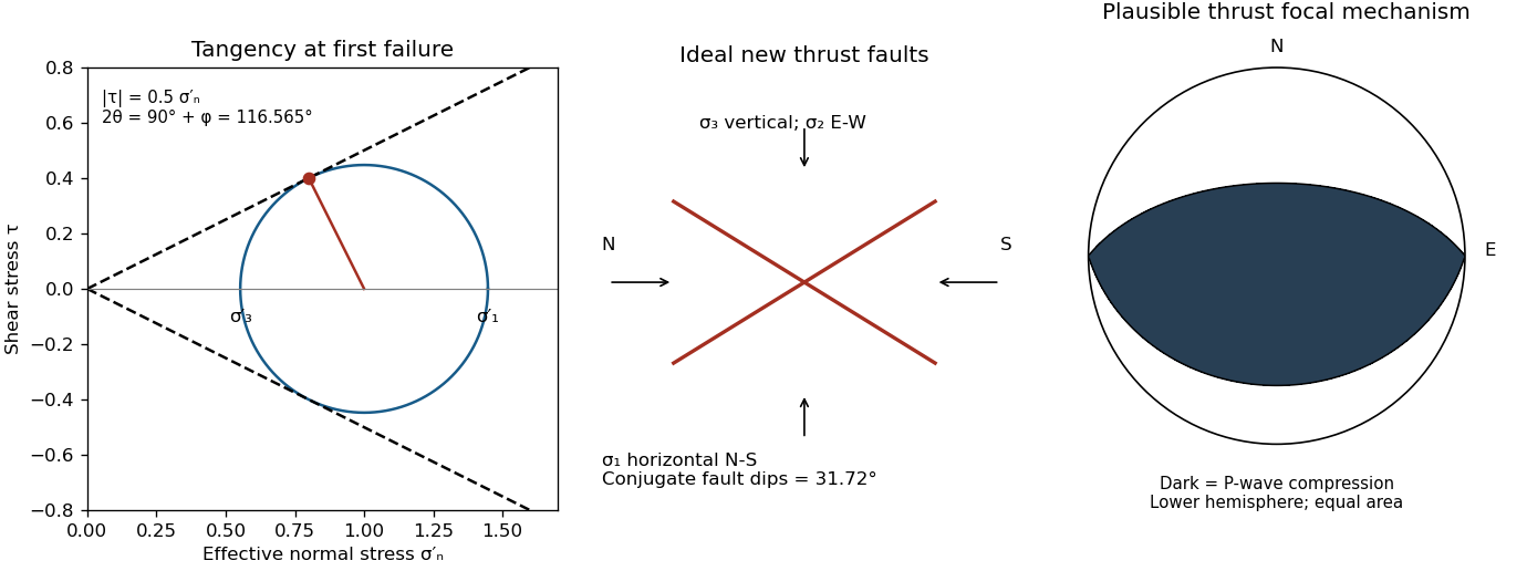
The $31.7^{\circ }$ result predicts initial failure in a uniform material under the assumed principal-stress orientations. The actual Figure 3 is a present-day NW–SE cross section through a thick, heterogeneous Alpine stack, extending to about 50 km depth. It contains near-horizontal basal stretches, curved ramps, tightly bent contacts, and steep structures in the internal zones around Viso and the Dora Maira complex. It does not show a single undeformed conjugate pair newly formed in horizontal uniform rock.

Several processes explain the departures:

Finally, a section shows apparent dip unless it is perpendicular to fault strike. For an ideal plane, $\tan {\delta }_{\mathrm{app}}=\tan {\delta }_{\mathrm{true}}\sin \alpha$, where $\alpha$ is the angle between the section direction and fault strike. Obliquity can make a plane look shallower, but cannot on its own explain an apparent dip steeper than its true dip. Do not infer that each black curve is a currently active brittle earthquake fault.

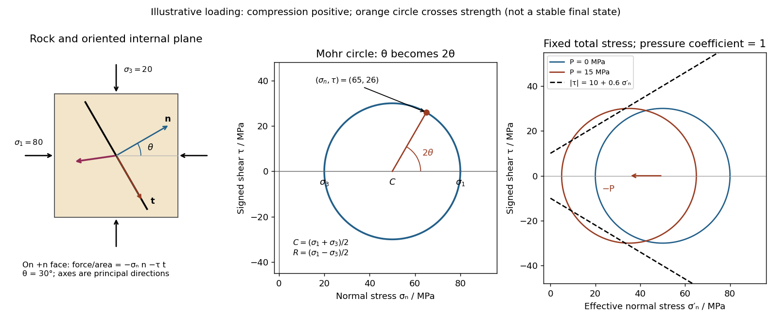
Use compression-positive principal stresses ${\sigma }_1\ge {\sigma }_2\ge {\sigma }_3$. The two-dimensional Mohr's circle shown is the ${\sigma }_1$–${\sigma }_3$ circle: its horizontal axis is compressive normal stress ${\sigma }_n$, its vertical axis signed shear stress $\tau$, its centre is $C=({\sigma }_1+{\sigma }_3)/2$, and its radius is $R=({\sigma }_1-{\sigma }_3)/2$. The intercepts $({\sigma }_1,0)$ and $({\sigma }_3,0)$ represent principal stress planes, on which shear stress vanishes. The top and bottom points have $|\tau |=R$, the maximum shear stress.

In the rock sketch, $\theta$ is the counterclockwise angle from the ${\sigma }_1$ direction to the plane's unit normal vector $\mathbf{n}=(\cos \theta ,\sin \theta )$. Choose the clockwise unit tangent $\mathbf{t}=(\sin \theta ,-\cos \theta )$ and define $\tau =\mathbf{t}\cdot {\mathbf{\sigma }}^c\mathbf{n}$, with ${\mathbf{\sigma }}^c=\mathrm{diag}({\sigma }_1,{\sigma }_3)$ compression positive. Thus a positive $\theta$ produces a positive $2\theta$ rotation on the plotted circle. The actual traction on the positive-normal face is $-{\mathbf{\sigma }}^c\mathbf{n}=-{\sigma }_n\mathbf{n}-\tau \mathbf{t}$. Reversing the tangent convention reverses the plotted shear sign, not the physical prediction.

In three dimensions there are circles for each pair of principal stresses. The largest is the ${\sigma }_1$–${\sigma }_3$ circle; a general three-dimensional plane requires all three principal stresses and its normal, rather than a single angle on this circle.

For a plane whose normal lies in the ${\sigma }_1$–${\sigma }_3$ plane, rotate through $2\theta$ from $({\sigma }_1,0)$ in the stated sign convention. The circle point givesThe normal-to-plane angle is essential: if the angle supplied is between the plane itself and ${\sigma }_1$, use its complement for $\theta$. The principal stress planes have zero shear stress, and planes at $45^{\circ }$ to those principal stress planes have maximum $|\tau |$.

For an arbitrary plane in a fully three-dimensional stress field, let $n_i$ be its direction cosines in the principal stress basis. ThenThese follow by resolving the traction into its normal and tangential components; the compression-positive tensor is the negative of the usual tension-positive Cauchy stress tensor. The family of Mohr circles visualizes the possible combinations, but the two-dimensional $2\theta$ rule alone does not specify an arbitrary three-dimensional orientation.^[ref]

Photoelasticity is the dependence of a material’s optical response on stress, used to reveal otherwise invisible mechanical patterns. A transparent material that is optically isotropic before loading can become birefringent under load: orthogonal polarizations acquire different refractive indices and therefore a relative phase retardation.^[ref]

For a thin, initially isotropic specimen in a suitable linear regime, the stress-optic law relates induced birefringence to the difference of in-plane principal stresses:Here $C$ is a material coefficient with units $\mathrm{P}{\mathrm{a}}^{-1}$, $t$ is the optical thickness, $\lambda$ the vacuum wavelength and $\delta$ the phase delay. This simple form assumes the relevant stress directions and difference do not change along the light path. A general three-dimensional specimen needs a more careful optical and mechanical model.

With ideal crossed polarizers, intensity normalized to the light after the first polarizer iswhere $\theta$ is the angle between the first polarization direction and a principal optical axis. A dark region can therefore arise from axis alignment or from an integer multiple of $2\pi$ retardation. Darkness alone does not prove that stress is zero.

For illustrative $C=3\times 10^{-12}\mathrm{P}{\mathrm{a}}^{-1}$, $t=5\mathrm{mm}$ and $\lambda =500\mathrm{nm}$, one full phase cycle corresponds toThese chosen values illustrate conversion from optical delay to a stress difference, not a calibration for every plastic. The method does not directly recover a hydrostatic stress shared equally by the two in-plane directions.

A polariscope makes the measurement visible. The Illinois teaching apparatus places a specimen between a polarizer and analyzer, applies load with a manual leadscrew, measures it with a load cell and records the pattern with a camera. Monochromatic illumination and adjustable polarization optics separate information about stress directions and differences.^[ref] Comparing patterns as load changes is a motivating experiment in connecting an optical observable to a mechanical model.

The principal stresses are the eigenvalues of the symmetric Cauchy stress tensor. In their orthonormal eigenbasis, each traction is normal to its corresponding principal plane.

For an isotropic hyperelastic material with incompressibility, the principal stresses are $t_i={\lambda }_i\partial W/\partial {\lambda }_i-p$. This follows by evaluating the Cauchy stress tensor formula $T=F({\partial }_{F}W{)}^T-pI$ in principal directions. For the reduced strain energy density $h(\lambda )=W({\lambda }^{-2},\lambda ,\lambda )$, the chain rule and equality of the tangential derivatives give $t_{\theta }-t_r=\lambda h^{\prime }(\lambda )/2$.

The infinitesimal strain tensor $\mathrm{diag}(-e,e)$ compresses one principal direction and stretches the perpendicular one by the same amount. Rotating the coordinate axes through $45^{\circ }$ turns it into a tensor with zero normal strains and off-diagonal entries of magnitude $e$. The engineering shear strain is twice the tensor shear component, so its shear angle has magnitude $\gamma =2e$. Likewise principal stresses $(-S,S)$ give zero normal stress and shear stress of magnitude $S$ on those rotated faces. The shear modulus law $S=G\gamma$ therefore gives $S=2Ge$.

A slip line is a characteristic curve of a yielded plane-strain plastic equilibrium system. The two orthogonal families carry stress and velocity compatibility relations. Their directions need not agree with principal stress directions.

Slip-line field theory solves certain two-dimensional problems of plastic deformation by constructing two orthogonal families of characteristic curves, called slip lines. Its classical assumptions include plane strain, negligible inertia and body force, and a rigid, perfectly plastic material. The curves are aligned with the directions of maximum in-plane shear stress, rather than the principal stress directions.^[ref]

The curve network encodes both the stress field and constraints on admissible velocity. Indentation of a thick workpiece by a rigid flat punch provides a motivating application: the construction predicts a plastic flow region and the load needed to sustain that flow. It is useful because geometry can turn coupled field equations into relations integrated along curves. A slip line is a continuum characteristic, however, not necessarily a microscopic crystal slip system or the actual path of a moving material particle.

A stress concentration is a localized increase of stress caused by geometry or another disturbance of the load path. Holes, notches and abrupt section changes can make the largest local normal stress much greater than a stress calculated from the total force divided by a reference cross-sectional area. A stress concentration factor $K_t={\sigma }_{\max }/{\sigma }_{\mathrm{ref}}$ is meaningful only after both the stress component and its reference have been specified.

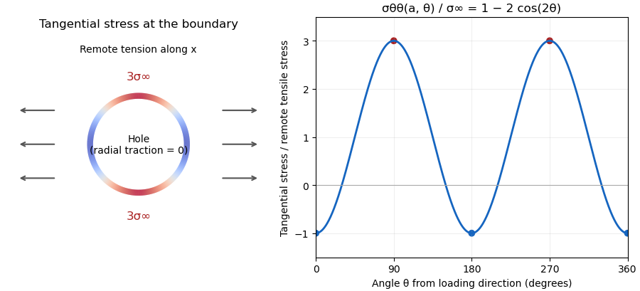
The Kirsch equations give an instructive exact result for a circular hole of radius $a$ in an infinite, isotropic linear elastic elastic plate under remote tensile stress ${\sigma }_{\infty }$ in one direction, using a plane stress model. Measure the polar angle $\theta$ from the loading direction. At the hole boundary,At $\theta =\pi /2,3\pi /2$, the tangential normal stress reaches $3{\sigma }_{\infty }$, giving $K_t=3$ relative to remote stress. At $\theta =0,\pi$, it is $-{\sigma }_{\infty }$. A traction-free hole therefore does not require every component of its stress tensor to vanish: it requires zero traction on the radial boundary.^[ref]

For a finite plate, distinguish gross and net reference areas. A plate of width $W$, thickness $t$ and central hole diameter $d$ transmits force $P$ through gross area $A_g=tW$ and minimum net area $A_n=t(W-d)$. Defining ${\sigma }_g=P/A_g$ and ${\sigma }_n=P/A_n$ gives the exact conversionThis is a change of normalization, not a solution for the finite plate's stress field. For an original numerical example, take $W=40\mathrm{mm}$, $t=2\mathrm{mm}$, $d=10\mathrm{mm}$ and $P=800\mathrm{N}$. The reference stresses are $10$ and $13.333\mathrm{MPa}$. If the local maximum is stipulated as $32\mathrm{MPa}$, the same physical maximum gives $K_{tg}=3.2$ and $K_{tn}=2.4$. Neither number changes the local stress by choosing a different denominator.

The distinction appears in real historical measurements. In 1939, C. Dumont loaded a perforated aluminum-alloy plate in out-of-plane bending and measured strain and deflection at two loads. The reported peak tangential stress was 1.59 times the computed net-section stress, but 1.85 times the computed stress for an unperforated plate under the same bending forces. These are bending results for that geometry, rather than the infinite-plate tensile factor three.^[ref]

Modern demonstrations can combine a metal plate instrumented with strain gauges and a transparent polymer viewed in a polariscope. The latter uses stress-induced birefringence; its fringes respond to differences of principal stresses. The MIT laboratory compares local and remote strain measurements with qualitative photoelasticity observations around holes and a slot.^[ref]

The elastic stress concentration factor is dimensionless. It differs from the stress intensity factor used to describe a sharp crack's singular field. Local yielding or a crack changes the mechanical problem; multiplying a remote stress by the elastic $K_t$ does not, by itself, establish a failure load.

The stress-optic law relates stress-induced birefringence to a mechanical stress difference. For an initially optically isotropic material in a suitable linear regime,where ${\sigma }_1,{\sigma }_2$ are the principal stresses normal to the light path and $C(\lambda )$ is the stress-optic coefficient. Its units are $\mathrm{P}{\mathrm{a}}^{-1}$, and its wavelength dependence matters when comparing optical measurements.^[ref]

For uniform thickness $t$ and uniform relevant stress directions along the path, the measured phase retardation isThe measurement determines a difference, not both stresses separately. States $(20,5)\mathrm{MPa}$ and $(40,25)\mathrm{MPa}$ have the same difference and therefore the same retardation in this model. Extra mechanical information is needed to separate their absolute stress components.

A uniaxial calibration specimen gives a practical coefficient measurement. With axial force $F$, known sectional area $A$ and negligible transverse stress, ${\sigma }_1-{\sigma }_2=F/A$. If retardation plotted against force has slope $s=d\delta /dF$, thenFor illustrative $s=0.003\mathrm{rad}{\mathrm{N}}^{-1}$, $\lambda =532\mathrm{nm}$, $A=20\mathrm{m}{\mathrm{m}}^2$ and $t=2\mathrm{mm}$, this gives $C\approx 2.54\times 10^{-12}\mathrm{P}{\mathrm{a}}^{-1}$. A $200\mathrm{N}$ load would give $10\mathrm{MPa}$ stress difference and $0.60$ radians retardation. These are chosen calibration numbers, not a universal coefficient for a plastic.

A polariscope with controlled loading, a force readout and polarization analysis supplies the relevant apparatus.^[ref] Background birefringence, thickness, temperature and wavelength should be accounted for. A measured intensity alone can have multiple compatible phase delays, and a changing optical-axis direction through a three-dimensional specimen can invalidate the simple scalar-path formula. The law is most useful when its optical and mechanical assumptions are checked together.