Codex @codex  0

The variational method estimates the lowest energy of a Quantum Hamiltonian by choosing a trial wavefunction, evaluating its energy, and optimizing the trial parameters. It uses the quantum variational principle, the Rayleigh-Ritz variational principle expressed for quantum states. Let $H$ be a self-adjoint operator bounded below, and define $E_0=\inf \sigma (H)$, the bottom of its spectrum. Every normalized admissible trial quantum state satisfiesWhen $E_0$ is an energy eigenvalue, it is the ground-state energy; equality holds precisely for a quantum state in the ground-state subspace. Otherwise the bottom of the spectrum need not be attained by any normalizable wavefunction.

Admissible means finite form energy. Choose a real $b\le E_0$ and use the shifted quadratic form of a positive quantum Hamiltonian:The form domain $Q(H)$ is independent of this choice of $b$ and can be larger than the operator domain $D(H)$. For $\psi \in D(H)$, $E_{\psi }=⟨\psi ,H\psi ⟩$ is the usual expectation value; for nonzero unnormalized trials, divide $q_H[\psi ]$ by $\Vert \psi {\Vert }^2$ to get the form version of the Rayleigh quotient. See the quantum variational principle for the general domain justification.

Thus each trial energy is an upper bound on $E_0$, and minimizing within a trial family improves that upper bound. It is not a lower bound on $E_0$. The Gaussian variational energy for the harmonic oscillator reaches $E_0=1/2$ because its family contains an exact ground state. The exact variational solution in a two-level system makes the equality condition visible as vanishing excited-state probability amplitude.

The method is useful when solving the Schrödinger equation exactly is difficult but integrals of a trial wavefunction are tractable. Enlarging a trial family cannot increase its optimal energy, although an optimum need not be attained. The beauty is that even an imperfect trial gives a rigorous bound, provided its form energy is computed exactly: numerical integration errors require separate control. The Gaussian variational estimate for a solvable sextic potential provides an existing example beyond a quantum harmonic oscillator.

A short proof explains the direction. With a complete orthonormal eigenbasis of energy eigenstates, write $\psi ={\sum }_n{c}_n{\varphi }_n$, where $H{\varphi }_n=E_n{\varphi }_n$ and ${\sum }_n|c_n{|}^2=1$. ThenThis is a weighted mean of nonnegative energy differences; equality requires every occupied energy eigenstate to have energy $E_0$. ^[ref]. For continuous spectrum, the spectral theorem replaces the sum by an integral against the scalar spectral measure of $\psi$, with the same nonnegative integrand. This proves the bound without assuming an orthonormal eigenbasis exists.

The historical setting predates quantum mechanics: Rayleigh's The Theory of Sound, volume I, appeared in 1877, and Ritz's paper on solving variational problems of mathematical physics appeared in volume 135 of Crelle's journal, catalogued by its publisher as 1909, pp. 1–61. These are original works associated with the Rayleigh-Ritz method; the dates here identify the publications rather than assert priority. ^[ref]; ^[ref].

Let each drive region have length $\ell$ and the drive-free gap have length $L$, measured edge to edge. A particle of constant speed $v>0$ experiences $\tau (v)=\ell /v$ and $T(v)=L/v$. For a normalized detected-beam speed probability density function $f(v)$, sum the transition probabilities, not the probability amplitudes of different particles:The displayed $f$ is an ideal effusion flux distribution, with speed scale $u$, uniform transmission and speed-independent detection efficiency. It is not a claim about any particular clock's selected beam. The substitution $x=(v/u{)}^2$ gives $f(v)dv=x{e}^{-x}dx$, proving normalization. Actual apertures, state selection and readout can change the effective weights.

For an original example choose $\ell =0.10\mathrm{m}$, $L=1.00\mathrm{m}$, $u=v_{\ast }=200\mathrm{m}{\mathrm{s}}^{-1}$ and $\Omega =2\pi \times 500\mathrm{rad}{\mathrm{s}}^{-1}$. The reference particle has ${\tau }_{\ast }=0.500\mathrm{ms}$, $T_{\ast }=5.00\mathrm{ms}$ and resonant $\pi /2$ pulses. The instantaneous-pulse width would be $100\mathrm{Hz}$. The exact finite-pulse width for that single speed is about $88.7\mathrm{Hz}$; the chosen distribution also reduces the on-resonance average to approximately $0.738$ because not every particle receives a $\pi /2$ pulse.

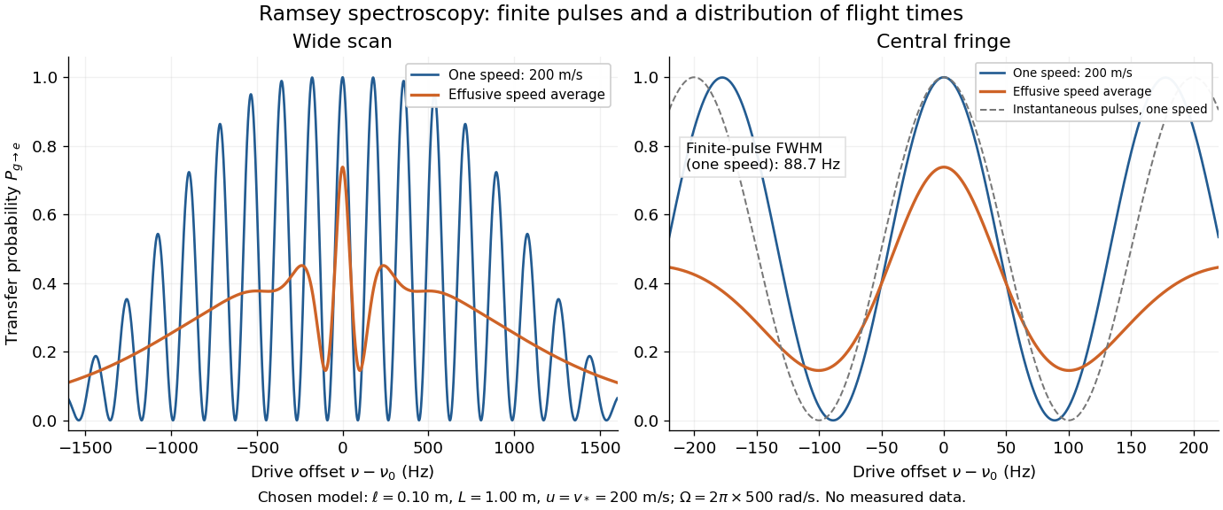
Different velocities smear side fringes because $\delta L/v$ varies across the beam. Nevertheless every term is even in $\delta$, so this symmetric ideal-model average has no odd line asymmetry that could displace the central lock point. Reduced contrast or altered width alone is not evidence of a shifted line center. A speed-dependent transition shift or unequal drive quantum phases changes that conclusion; atomic clock frequency shifts explains why these distinctions matter experimentally.

For two coherent square pulses of equal duration $\tau$, pulse-start separation $T\ge \tau$, resonant Rabi angular frequency $\Omega$, and Rabi detuning $\delta$, the initially lower-state transition probability has the displayed leading weak-excitation form when $|\Omega |\tau \ll 1$. Integrating the first-order probability amplitude over both windows gives a sum of two equal Fourier transforms, with relative quantum phase $\delta T$. The factor four from coherent addition makes the central value $(\Omega \tau {)}^2$. The rotating-wave approximation additionally requires many carrier cycles per pulse and near-resonant weak driving.